CFA L2 2024 Volume 1 - Quantitative Methods

Quantitative Methods Learning Module 1 Basics of Multiple Regression and Underlying Assumptions LOS: Describe the types of investment problems addressed by multiple linear regression and the regression process. LOS: Formulate a multiple linear regression model, describe the relation between the dependent variable and several independent variables, and interpret estimated regression coefficients. LOS: Explain the assumptions underlying a multiple linear regression model and interpret residual plots indicating potential violations of these assumptions. Multiple linear regression is a modeling technique that uses two or more independent variables to explain the variation of the dependent variable. A reliable model can lead to a better understanding of value drivers and improve forecasts, but an unreliable model can lead to spurious correlations and poor forecasts. Several software programs and functions exist to help execute multiple regression models: Software Programs/Functions Excel Data Analysis > Regression scipy.stats.linregress Python statsmodels.lm sklearn.linear_model.LinearRegression R lm PROC REG PROC GLM SAS STATA regress Vol 1-3 Learning Module 1 Uses of Multiple Linear Regression LOS: Describe the types of investment problems addressed by multiple linear regression and the regression process. The complexity of financial and economic relationships often requires understanding multiple factors that affect the dependent variable. Some examples where multiple linear regression can be useful include: y A portfolio manager wants to understand how returns are influenced by underlying factors. y A financial advisor wants to identify when financial leverage, profitability, revenue growth and changes in market share can predict financial distress. y An analyst wants to examine the effect of country risk on fixed-income returns. In all cases, the basic framework of a regression model is as follows: y Specify a model, including independent variables. y Estimate a regression model and analyze it to ensure that it satisfies key underlying assumptions and meets the goodness-of-fit criteria. y Test the model’s out-of-sample performance. If acceptable, it can then be used for further identifying relationships between variables, testing existing theories, or forecasting. Vol 1-4 Basics of Multiple Regression and Underlying Assumptions Exhibit 1 Regression process Explain the variation of the dependent variable by using the variation of other, independent variables Is the dependent variable continuous? Use logistic regression No Yes Estimate the regression model Analyse the residuals Are the assumptions of regression Adjust the model No satisfied? Yes Examine the goodness of fit of the model Is the overall fit significant? No No Yes Is the model the best of possible models? Yes Use the model for analysis and prediction © CFA Institute Vol 1-5 Learning Module 1 The Basics of Multiple Regression LOS: Formulate a multiple linear regression model, describe the relation between the dependent variable and several independent variables, and interpret estimated regression coefficients. Multiple regression is similar to simple regression where a dependent variable, Y, is explained by the variation of an independent variable, X. Multiple regression expands this concept into a statistical procedure that evaluates the impact of more than one independent variable on a dependent variable. A multiple linear regression model has the following general form: Multiple regression equation Yi = b0 + b1X1i + b2X2i + ∙∙∙ + bkXki + ε i , i = 1, 2, ..., n Where: Yi = The ith observation of the dependent variable Y X = The ith observation of the independent variable X , j = 1, 2, …, k ji j b = The intercept of the regression 0 b , …, b = The slope coefficients for each of the independent variables 1 k ε i = The error term for the ith observation n = The number of observations The slope coefficients, b to b , measure how much the dependent variable, Y, changes in response to 1 k a one-unit change in that specific independent variable. In our equation, the independent variable X , 1 holding all other independent variables constant, will change Y by a factor of b . Here, b is called a partial 1 1 regression coefficient, or a partial slope coefficient, because it explains only the part of the variation in Y related to that specific variable, X . 1 Note that for any multiple regression equation: y There are k slope coefficients in a multiple regression. y The k slope coefficients and the intercept, b , are all known as regression coefficients. 0 y There are k + 1 regression coefficients in a multiple regression equation. y The residual term, ε , equals the difference between the actual value of Y (Y ) and the predicted value i i Residual term i i 1i 2i ki Vol 1-6 of Y (5). In terms of our multiple regression equation: i i ε̂ = Y − 5 = Y − (3 + 3 X + 3 X + ∙∙∙ + 3 X ) i 0 1 2 k Basics of Multiple Regression and Underlying Assumptions Assumptions Underlying Multiple Linear Regression LOS: Explain the assumptions underlying a multiple linear regression model and interpret residual plots indicating potential violations of these assumptions. In order to make valid predictions using a multiple regression model based on ordinary least squares (OLS), a few key assumptions must be met. Exhibit 2 Multiple linear regression assumptions Assumption Description Violation Dependent and independent variable have linear relationship Linearity Nonlinearity Variance of residuals constant across all observations Homoskedasticity Independence of errors Normality Heteroskedasticity Observations are independent of each other; errors (ie, residuals) uncorrelated across all observations Serial correlation or autocorrelation Residuals normally distributed, with expected value of zero Non-normality Independent variables are not random; no exact linear relation between independent variables Independence of independent variables Multicollinearity Statistical tools exist to test these assumptions and the model for overall goodness of fit. Most regression software packages have built in diagnostics for this purpose. To better illustrate this, consider a regression to analyze 10 years of monthly total excess returns of ABC stock using the Fama-French three-factor model. This model uses market excess return (MKTRF), size (SMB), and value (HML) as explanatory variables. ABC = b + b MKTRF + b SMB + b HML + ε return 0 1 t 2 t 3 t t t Vol 1-7 Learning Module 1 The software produced the following set of scatterplots to test the relationship between the three independent variables: Exhibit 3 Scatterplots for three independent variables 0.06 0.04 0.02 0.02 −0.02 −0.04 0.05 0.00 −0.05 −0.10 −0.15 0.2 0.1 0.0 −0.1 −0.2 −0.10 0.00 0.10 −0.05 0.00 SMB 0.05 −0.1 0.00 HML −0.2 0.0 0.2 MKTRF ABC_RETRF © CFA Institute In the lower set of scatterplots of Exhibit 3, there is a positive relationship between ABC’s return and the market risk factor (MKTRF), no apparent relationship between ABC’s return and the size factor (SMB) and a negative relationship between ABC’s return and the value factor (HML). In the second-to-last (penultimate) level we can see little relationship between SMB and HML. This suggests independence between the variables, which satisfies the assumption of independence. t in Exhibit 4: Vol 1-8 Then, compare the predicted values, or 5, with the actual values of ABC RETRF in the residual plot i Basics of Multiple Regression and Underlying Assumptions Exhibit 4 Residual plot 0.20 0.15 0.10 0.05 0.00 −0.05 −0.10 −0.15 −0.20 −0.25 −0.15 −0.1 −0.05 0 0.05 0.1 0.15 0.2 Predicted value Potential outliers indicated with square markers © CFA Institute Exhibit 4 shows the relationship between the residuals and the predicted values. A visual inspection does not show any directional relationship, positive or negative, between the residuals and the predicted values from the regression model. This also suggests that the regression’s errors have a constant variance and are uncorrelated with each other. There are however, three residuals (square markers) that may be outliers. Vol 1-9 Learning Module 1 Exhibit 5 Regression residuals versus each of the three factors 0.20 0.15 0.10 0.05 0.00 −0.05 −0.10 −0.15 −0.20 −0.25 −0.06 −0.4 −0.02 0.00 0.02 0.04 0.06 0.08 0.08 0.10 MKTRF 0.20 0.15 0.10 0.05 0.00 −0.05 −0.10 −0.15 −0.20 −0.25 −0.06 −0.4 −0.02 0.00 0.02 0.04 0.06 SMB 0.20 0.15 0.10 0.05 0.00 −0.05 −0.10 −0.15 −0.20 −0.25 −0.20 −0.15 −0.10 −0.05 0.00 0.05 HML © CFA Institute Vol 1-10 Basics of Multiple Regression and Underlying Assumptions Each plot shows the relationship of the residual output versus the value of each independent variable to look for directional relationships related to that specific factor. In this example, none of the three plots indicate any direct relationship between the residuals and the explanatory variables, which suggests that there is no violation of multiple regression assumptions. Furthermore, in all four graphs, the outliers identified are the same. Exhibit 6 is a normal Q-Q plot used to visualize the distribution of a variable compared with a theoretical normal distribution. Exhibit 6 0.20 0.15 0.10 0.05 0.00 −0.05 −0.10 −0.15 −0.20 −0.25 −3 −2 −1 0.00 1 2 3 Theoretical distribution Superimposed on the plot is a linear relation © CFA Institute In this plot, the red line represents a normal distribution with a mean of 0 and a standard deviation of 1. The green dots are the model residuals fit to a normal distribution, or the empirical distribution on the vertical axis of Exhibit 5. These are superimposed over the red theoretical distribution line to visualize how consistent the normalized residuals are with a standard normal distribution. The same three outliers remain, but the rest of the residuals closely align with a normal distribution, which is the desired outcome. Vol 1-11 Learning Module 1 Vol 1-12 Learning Module 2 Evaluating Regression Model Fit and Interpreting Model Results LOS: Evaluate how well a multiple regression model explains the dependent variable by analyzing ANOVA table results and measures of goodness of fit. LOS: Formulate hypotheses on the significance of two or more coefficients in a multiple regression model and interpret the results of the joint hypothesis tests. LOS: Calculate and interpret a predicted value for the dependent variable, given the estimated regression model and assumed values for the independent variable. Goodness of Fit LOS: Evaluate how well a multiple regression model explains the dependent variable by analyzing ANOVA table results and measures of goodness of fit. T 2 he coefficient of determination measures a regression’s goodness of fit, known as the R statistic: how much of the variation in the dependent variable is captured by the independent variables in the regression. Exhibit 1 shows how a regression model explains the variation in the dependent variable: Exhibit 1 Regression model seeks to explain the variation of Y Total variation of Y Sum of squares Variation of Y explained regression (SSR) by the regression n 2 (Y − Y) Sum o i f squares i = 1 total (SST) n 2 (Y − Y) i Sum of squares Variation of Y unexplained i = 1 error (SSE) by the regression n 2 (Y − Y ) i i i = 1 Y = Dependent variable Y = Predicted value of Y for a particular X i i Yi = Observed value of Y for a particular Xi Y = Average value of Y Vol 1-13 Learning Module 2 R2 is calculated as: Coefficient of determination R2 = Total variation − Unexplained variation Sum of squares regression R2 = Sum of squares total n n R2 2 2 = (Y − Y ) / (Y − Y ) i i i i i = 0 i = 0 Where: n is the number of observations in the regression Yi is an observation of the Y variable Y is the predicted value of the dependent variable Y is the average of the dependent variable A ma 2 jor concern with using R in multiple regression analysis is that as more independent variables are added to the model, the total amount of unexplained variation will decrease as the amount of explained va 2 riation increases. As such, each successive R measure will appear to reflect an improvement over the previous model. This will be the case as long as each newly added independent variable is even slightly correlated with the dependent variable and is not a linear combination of the other independent variables already in the regression model. O 2 ther limitations to using R : y It does not tell the analyst whether the coefficients are statistically significant y It does not indicate whether there are biases in the coefficients or predictions y It can misread the fit due to bias and overfitting Overfitting can result from an overly complex model with too many independent variables relative to the number of observations. In such cases, the model does not properly represent the true relationship between the independent and dependent variables. 2 Therefore, analysts typically use adjusted R , or 7 , which does not increase whenever another variable is 2 added to the regression since it is adjusted for degrees of freedom. A 2 djusted R Sum of squares error / (n − k − 1) R2 = Sum of squares total / (n − k − 1) Where: k = Number of independent variables 2 A few things to note when comparing R to 72 2 y If k = 1, R > 72 y 72 will decrease if the inclusion of another independent variable in the regression model results in a nominal increase in explained variation (RSS) and R2. Vol 1-14 Evaluating Regression Model Fit and Interpreting Model Results 2 y 7 can be negative (in which case we consider its value to equal 0) while R can never be negative. 2 y If 7 is used to compare two regression models, the dependent variable must be identically defined in 2 the two models and the sample sizes used to estimate the models must be the same. | | 2 | | 2 Additionally, if the t-statistic > 1 then 7 will increase; conversely, values < 1 will decrease 7 2 There are cases where both the R and 7 can increase when more independent variables are added. For 2 these cases there are several statistics used to compare model quality, including Akaike’s information criterion (AIC) and Schwarz’s Bayesian information criterion (BIC). AIC is used to evaluate a collection of models that explain the same dependent variable. Even though this will generally be provided in the output for regression software, we can also calculate it as: Sum of squares error AIC = n × ln + 2(k + 1) n Where: k = Number of independent variables n = Sample size A lower AIC indicates a better-fitting model. Note that AIC depends on the sample size (n), the number of independent variables (k), and the sum of the squares error (SSE). The term at the end, 2(k + 1), is a penalty term that increases as more independent variables, k, are added. Similarly, BIC allows comparison of models with the same dependent variable: Sum of squares error BIC = n × ln + ln(n)(k + 1) n Where: k = Number of independent variables n = Sample size With BIC, there is a greater penalty for having more parameters than with AIC. BIC will tend to prefer smaller models because ln(n) is greater than 2, even for very small sample sizes. AIC is preferred if the model is for prediction purposes, and BIC is preferred for evaluating goodness of fit. Vol 1-15 Learning Module 2 The AIC and the BIC alone are not telling, however, and should be compared across models using a combination of factors. Example 1 shows the goodness-of-fit measures for a model that incorporates five independent variables (factors): Example 1 Goodness of fit evaluation R2 Ad 2 justed R AIC BIC Factor 1 only 0.541 0.541 0.562 0.615 0.615 0.531 0.531 0.533 0.580 0.572 19.079 21.078 20.743 16.331 18.251 22.903 26.814 28.393 25.891 29.687 Factors 1 and 2 Factors 1, 2, and 3 Factors 1, 2, 3, and 4 Factors 1, 2, 3, 4, and 5 Note that: R2 increases or stays the same as more factors are added 72 either increases or decreases as each new factor is added AIC is minimized when the first four factors are used BIC is minimized when only the first is used Using the results, we would select the four-factor model if we were using it to make predictions, but would use the first model if we were just measuring goodness of fit. Testing Joint Hypotheses for Coefficients LOS: Formulate hypotheses on the significance of two or more coefficients in a multiple regression model and interpret the results of the joint hypothesis tests. In a multiple regression, the intercept is the value of the dependent variable if all independent variables are 0. The slope coefficient of each of the independent variables is the change in the dependent variable for a change in that independent variable if all other independent variables remain constant. Tests for individual coefficients in multiple regression are identical to tests for individual coefficients in simple regression. The hypothesis structure is the same and the t-test is the same. For a two-sided test of whether a variable is significant in explaining the dependent variable’s variation, the hypotheses are: H0 : bi = Bi Ha : bi ≠ Bi Where b is the true coefficient for the ith independent variable and B is a hypothesized slope coefficient for the same variable. Vol 1-16 Evaluating Regression Model Fit and Interpreting Model Results If the hypothesis test is simply to test the significance of the variable’s predictive power, the hypotheses would be: H : B = 0 and H : B ≠ 0 0 j a j There are times to test a subset of variables in a multiple regression, for example, when comparing the HML, RMW, CMA) to determine which model is more concise or to find the factors that are most useful in explaining the variation in the dependent variable. In other words, it may be that not all the factors in such a model are actually required for the model to have predictive power. The full model, using all independent variables, is called the unrestricted model. This model is compared with a restricted model, which effectively includes fewer independent variables since coefficients for each unneeded variable are set to 0. A restricted model is also called a nested model since its independent variables form a subset of the variables in the unrestricted model. Unrestricted five-factor model: Y = b b X b X b X b X b X ε i 0 + 1 1i + 2 2i + 3 3i + 4 4i + 5 5i + i Restricted two-factor model: Y = b + b X + b X + ε i 0 1 1i 4 4i i The hypothesis test in this example would be to test whether the coefficients of X , X , and X are 2 3 5 significantly different than 0. To compare the unrestricted model to the nested model, perform an F-test to test the role of the jointly omitted variables: Sum of squares error − Sum of squares error (Restricted model) (Unrestricted model) q F = Sum of squares error (Restricted model) n − k − 1 Where: q = Number of variables omitted in the restricted model The role of the F-test determines whether the change in the sum of squared errors (SSE) caused by including the variables from the unrestricted model is significant enough to compensate for the decrease in degrees of freedom. In the example shown here, there is a loss of three degrees of freedom since there are only two independent variables instead of five. y The null hypothesis is that the slope of the omitted factors is equal to 0: y The alternative hypothesis is that at least one is not equal to 0: H : at least one of the factors ≠ 0. a If the F-statistic is less than the critical value, then we fail to reject the null hypothesis. This means that the added predictive power of the variables omitted in the restricted model is not significant and the restricted model fits the data better. Vol 1-17 Fama-French three-factor model (MKTRF, SMB, HML) to the Fama-French five-factor model (MKTRF, SMB, Learning Module 2 Exhibit 2 summarizes the desired values of a multiple regression test: Exhibit 2 Assessing model fit using multiple regression statistics Statistic Criterion to use in assessment The higher the better Ad 2 justed R Akaike’s information criterion (AIC) The lower the better Schwarz’s Bayesian information criterion (BIC) The lower the better Outside the bounds of critical t-value(s) for the selected significance level t-statistic on a slope coefficient Exceeds the critical F-value for the selected significance level F-test for joint tests of slope coefficients © CFA Institute Forecasting Using Multiple Regression LOS: Calculate and interpret a predicted value for the dependent variable, given the estimated regression model and assumed values for the independent variable. Predicting the value of the dependent variable in a multiple regression is similar to the prediction process for a simple regression. However, in the case of multiple independent variables, the predicted value is the sum of the product of each variable and its coefficient, plus the intercept: 5f = 30 + 31X1f + 32X2f + … 3kXkf For example, given the following formula: 5i = 3.546 + 3.235X1 + 7.342X2 − 7.234X3 Assume the values of X , X , and X are: 1 2 3 X1 X2 X3 3.8 8.3 5.9 With this information the predicted value of Y is calculated as: i 5 = 3.546 + (3.235 × 3.8) + (7.342 × 8.3) − (7.234 × 5.9) = 34.097 i Vol 1-18 Evaluating Regression Model Fit and Interpreting Model Results It should be noted that the estimate should include all the variables, even those that are not statistically significant, since these variables were used in estimating the value of the slope coefficient. As with simple linear regression, in multiple linear regression there will often be a difference between the actual value and the value forecasted by the regression model. This is the error term, or the ε1 term of the regression equation: the difference between the predicted value and the actual value. This is the basic uncertainty of the model known as the model error. Models using estimated independent variables add another source of error. These out-of-sample data introduce sampling error to the model and will increase the error contributed by the model error. Vol 1-19 Learning Module 2 Vol 1-20 Learning Module 3 Model Misspecification LOS: Describe how model misspecification affects the results of a regression analysis and how to avoid common forms of misspecification. LOS: Explain the types of heteroskedasticity and how it affects statistical inference. LOS: Explain serial correlation and how it affects statistical inference. LOS: Explain multicollinearity and how it affects regression analysis. Model Specification Errors LOS: Describe how model misspecification affects the results of a regression analysis and how to avoid common forms of misspecification. Model specification refers to the set of variables included in the regression and the regression equation’s functional form. A good regression model will: y y y y Be grounded in economic reasoning Be concise: each variable included in the model is essential Perform well out of sample Have an appropriate functional form (for example, if a nonlinear form is expected, then it should use nonlinear terms) y Satisfy regression assumptions, without heteroskedasticity, serial correlation, or multicollinearity Vol 1-21 Learning Module 3 Misspecified Functional Form Exhibit 1 illustrates four ways a model’s functional form may fail: Exhibit 1 Functional form failures Failures in regression Explanation Possible consequence functional form One or more important variables are Omitted variables Heteroskedasticity or omitted from the regression serial correlation Ignoring a nonlinear relationship Inappropriate form between the dependent and the of variables Heteroskedasticity independent variable One or more regression variables Inappropriate Heteroskedasticity or multicollinearity may need to be transformed before variable scaling estimating the regression Regression model pools data from different samples that should not be pooled Inappropriate data pooling Heteroskedasticity or serial correlation Omitted Variables The omitted variable bias is the bias resulting from the omission of an important independent variable. For example, assume the true regression model is defined as: Y = b + b X i + b X i + ε 1 0 1 1 2 2 i But the model was estimated as: Y = b + b X i ε 1 0 1 1 + i In this case, the model would be misspecified by the omission of X . If the omitted variable is uncorrelated 2 with X , then the residual would be b X i + ε . This means that the residual would not have an expected 1 2 2 value of 0 nor would it be independent and identically distributed. As a result, the estimate of the intercept 1 If, however, the omitted variable X is correlated with X , then the error term in the model would now be 2 1 correlated with X and the estimated values in the model would be biased and inconsistent with b , so the 1 1 intercept and residuals would also be incorrect. Inappropriate Form of Variables An example is when the analyst fails to account for nonlinearity in the relationship between the dependent variable and one or more independent variables. The analyst should consider whether the situation suggests a nonlinear relationship and should confirm nonlinearity by plotting the data. Sometimes, misspecification can be fixed by taking the natural logarithm of the variable. Vol 1-22 i would be biased, even if the X were estimated correctly. Model Misspecification Inappropriate Scaling of Variables Using unscaled data when scaled data is more appropriate can result in a misspecified model. This can happen, for example, when looking at financial statement data across companies. This misspecification can be addressed by using common-size financial statements, allowing analysts to quickly compare trends such Inappropriate Pooling of Data Inappropriate pooling of data occurs when a sample spans structural breaks in the behavior of the data, such as changes in government regulations or a change from a low-volatility period to a high-volatility period. In a scatterplot, this type of data can appear in discrete, widely separated clusters with little or no correlation. This can be fixed by using the subsample most representative of conditions during the forecasting period. Violations of Regression Assumptions: Heteroskedasticity LOS: Explain the types of heteroskedasticity and how it affects statistical inference. Heteroskedasticity occurs when the variance of the error term in the regression is not constant across observations; it results from a violation of the assumption of homoskedasticity, that is, that there is no systematic relationship between the regression residuals, or the vertical distances between the data points and the regression line, and the independent variable. Heteroskedasticity can result from any kind of model misspecification. Exhibit 2 shows the scatterplot and regression line for a model with heteroskedasticity. Notice that the regression residuals appear to increase in size as the value of the independent variable increases. Exhibit 2 Example of heteroskedasticity (violation of the homoskedasticity assumption) Linear regression Residual plot 25 20 120 100 80 15 10 5 0 60 50 100 150 200 250 −5 −10 −15 −20 −25 −30 40 20 0 50 X = Annual household income (USD thousands)(independent variable) 100 150 200 250 X = Annual household income (USD thousands) Vol 1-23 as profitability, leverage, and efficiency. Learning Module 3 Consequences of Heteroskedasticity Heteroskedasticity comes in two forms: y Unconditional heteroskedasticity occurs when the heteroskedasticity of the variance in the error term is not related to the independent variables in the regression. Unconditional heteroskedasticity does not create major problems for regression analysis even though it violates a linear regression assumption. y Conditional heteroskedasticity occurs when the heteroskedasticity in the error variance is correlated with the independent variables in the regression. While conditional heteroskedasticity creates problems for statistical inference, such as unreliable F-tests and t-tests, it can be easily identified and corrected. Conditional heteroskedasticity will tend to find significant relationships when none actually exist and lead to Type I errors, or false positives. Testing for Conditional Heteroskedasticity The most common test for heteroskedasticity is the Breusch-Pagan (BP) test. The BP test is best explained as a three-step process requiring a regression of the squared residuals from the original estimated regression equation, where the dependent variable is regressed on the independent variables in the regression. If conditional heteroskedasticity does not exist, the independent variables will not explain much of the variation in the squared residuals from the original regression. However, if conditional heteroskedasticity is present, the independent variables will explain the variation in the squared residuals to a significant extent. Because, in this case, each observation’s squared residual is correlated with the independent variables, the independent variable will affect the variance of the errors. The test statistic for the BP test is approximately chi-square distributed, and is calculated as: Chi-square test statistic X2 = nR2 Where: n = Number of observations R2 = Coefficient of determination of the second regression (the regression when the squared residuals of the original regression are regressed on the independent variables) k = Number of independent variables The null hypothesis is that the original regression’s squared error term is uncorrelated with the independent variables, or no heteroskedasticity is present. The alternative hypothesis is that the original regression’s squared error term is correlated with the independent variables, or heteroskedasticity is present. The BP test is a one-tailed chi-square test, because conditional heteroskedasticity is only a problem if it is too large. Vol 1-24 BP,k Model Misspecification Example 1 Testing for heteroskedasticity An analyst wants to test a hypothesis suggested by Irving Fisher that nominal interest rates increase by 1% for every 1% increase in expected inflation. The Fisher effect assumes the following relationship: i = r + πe Where: y i = Nominal interest rate y r = Real interest rate (assumed constant) y π = Expected inflation e The analyst specifies the regression model as: i = b + b π + ε . i 0 1 e i Since the Fisher effect basically asserts that the coefficient on the expected inflation (b ) variable equals 1 1, the hypotheses are structured as: H : b = 1 0 1 H : b ≠ 1 a 1 Quarterly data for 3-month T-bill returns, the nominal interest rate, are regressed on inflation rate expectations over the last 25 years. The results of the regression are: Coefficient Standard error t-statistic Intercept 0.04 1.153 0.029 0.45 0.0051 0.065 7.843 Expected inflation Residual standard error Multiple R-squared Observations 17.738 100 Durbin-Watson statistic 0.547 To determine whether the data support the assertions of the Fisher relation, we calculate the t-stat for the slope coefficient on expected inflation as: b − b 1.153 − 1 1 1 t = = ≈ 2.35 Standard error 0.065 b1 The critical t-values with 98 degrees of freedom at the 5% significance level are approximately −1.98 and +1.98. The test statistic is greater than the upper critical t-value, so we reject the null hypothesis and conclude that the Fisher effect does not hold, since the coefficient on expected inflation appears to be significantly different from 1. However, before accepting the validity of the results of this test, we should test the null hypothesis that the regression errors do not suffer from conditional heteroskedasticity. A regression of the squared 2 residuals from the original regression on expected inflation rates yields R = 0.193. Vol 1-25 Learning Module 3 The test statistic for the BP test is calculated as: Χ2 2 = nR = 100 × 0.193 = 19.3 T 2 he critical Χ value at the 5% significance level for a one-tailed test with one degree of freedom is 3.84. Since the t-statistic (19.3) is higher, we reject the null hypothesis of no conditional heteroskedasticity in the error terms. Since conditional heteroskedasticity is present in the residuals (of the original regression), the standard errors calculated in the original regression are incorrect, and we cannot accept the result of the t-test above (which provides evidence against the Fisher relation) as valid. Correcting Heteroskedasticity With efficient markets, heteroskedasticity should not exist in financial data. However, when it can be observed, an analyst should not only look to correct for heteroskedasticity, but also understand it and try to capitalize on it. There are two ways to correct for conditional heteroskedasticity in linear regression models. The first is to use robust standard errors, also known as White-corrected standard errors or heteroskedasticityconsistent standard errors, to recalculate the t-statistics for the original regression coefficients. The other method is to use generalized least squares, where the original regression equation is modified to eliminate Example 2 Using robust standard errors to adjust for conditional heteroskedasticity The analyst corrects the standard errors from the initial regression of 3-month T-bill returns (nominal interest rate) on expected inflation rates for heteroskedasticity and obtains the following results: Coefficient Standard error t-statistic Intercept 0.04 1.153 0.029 0.45 0.0048 0.085 8.333 Expected inflation Residual standard error Multiple R-squared Observations 13.565 100 Compared with the regression results in Example 1, notice that the standard error for the intercept does not change significantly, but the standard error for the coefficient on expected inflation increases by about 30% (from 0.065 to 0.085). Further, the regression coefficients remain the same (0.04 for the intercept and 1.153 for expected inflation). Using the adjusted standard error for the slope coefficient, the test statistic for the hypothesis test is calculated as: b − b 1.153 − 1 1 1 t = = ≈ 1.8 Standard error 0.085 b1 Vol 1-26 heteroskedasticity. Model Misspecification When we compare this test statistic to the upper critical t-value (1.98), we fail to reject the null hypothesis since the upper value is greater than the test statistic. The conditional heteroskedasticity in the data was so significant that the result of our hypothesis test changed once the standard errors were corrected for heteroskedasticity. We can conclude that the Fisher effect holds since the slope coefficient of the expected inflation independent variable does not significantly differ from 1. Violations of Regression Assumptions: Serial Correlation LOS: Explain serial correlation and how it affects statistical inference. Serial correlation (autocorrelation) occurs when regression errors are correlated, either positively or negatively, across observations, typically in time-series regressions. The Consequences of Serial Correlation Serial correlation results in incorrect estimates of the regression coefficients’ standard errors. If none of the regressors, or independent variables, is a lagged value of the dependent variable, it will not affect the consistency of the estimated regression coefficients. For example, when examining the Fisher relation, if we were to use the T-bill return for the previous month as an independent variable (even though the T-bill return that represents the nominal interest rate is actually the dependent variable in our regression model), serial correlation would cause all parameter estimates from the regression to be inconsistent. y Positive serial correlation occurs when: ○ a positive residual from one estimate increases the likelihood of a positive residual in the next observation. ○ a negative residual from one observation raises the probability of a negative residual resulting from the next observation. ○ In either case, positive serial correlation will result in a stable pattern of residuals over time. y Negative serial correlation occurs when a positive residual in one instance increases the likelihood of a negative residual in the next. Positive serial correlation is the most common type found in regression models. Positive serial correlation does not affect the consistency of the estimated regression coefficients, but it does have an impact on statistical tests. It will cause the F-stat, which is used to test the overall significance of the regression, to be inflated because MSE will tend to underestimate the population error variance. In addition, it will cause the standard errors for the regression coefficients to be underestimated, which results in larger t-values. Consequently, analysts may incorrectly reject null hypotheses, making Type I errors, and attach significance to relationships that are in fact not significant. Testing for Serial Correlation The Durbin-Watson (DW) test and the Breusch-Godfrey (BG) test are the most common tests for serial correlation. Vol 1-27 Learning Module 3 The DW test is a measure of autocorrelation that compares the squared differences of successive residuals with the sum of the squared residuals. This test is somewhat limited, however, because it only applies to first-order serial correlation. The BG test is more robust because it can detect autocorrelation up to a pre-designated order p, where the error in period t is correlated with the error in period t-p. The null hypothesis of the BG test is that there is no serial correlation in the model’s residuals up to lag p. The alternative hypothesis is that the correlation of residuals of at least one of the lags is different from zero and that serial correlation exists up to that order. The test statistic is approximately F-distributed with n-p-k-1 degrees of freedom where p is the number of lags. Correcting Serial Correlation There are two ways to correct for serial correlation in the regression residuals: 1. Adjust the coefficient standard errors to account for serial correlation: The regression coefficients remain the same but the standard errors change. This also corrects for heteroskedasticity. After correcting for positive serial correlation, the robust standard errors are larger than they were originally. Note that the DW stat still remains the same. 2. Modify the regression equation to eliminate the serial correlation. Example 3 Correcting for serial correlation The table shows the results of correcting the standard errors of the original regression for serial correlation and heteroskedasticity using Hansen’s method: Coefficient Standard error t-statistic Intercept 0.04 1.153 0.029 0.45 0.0088 0.155 4.545 Expected inflation 7.439 Residual standard error Multiple R-squared Observations 100 Durbin-Watson statistic 0.547 Note that the coefficients for the intercept and slope are exactly the same (0.04 for the intercept and 1.153 for expected inflation) as in the original regression (Example 1). Further, note that the DW stat is the same (0.547), but the standard errors have been corrected (they are now much larger) to account for the positive serial correlation. Given these new and more accurate coefficient standard errors, test the null hypothesis that the coefficient on the expected inflation independent variable equals 1. The test statistic for the hypothesis test is calculated as: b − b 1 1 t = = (1.153 − 1)/0.155 ≈ 0.98 Standard error b1 Vol 1-28 Model Misspecification The critical t-values with 98 degrees of freedom at the 5% significance level are approximately −1.98 and +1.98. Comparing the test statistic (0.987) with the upper critical t-value (+1.98) we fail to reject the null hypothesis and conclude that the Fisher effect holds as the slope coefficient on the expected inflation independent variable does not significantly differ from 1. Note that this result is different from the result of the test we conducted using the standard errors of the original regression (which were affected by serial correlation and heteroskedasticity) in Example 2. Further, the result is the same as from the test conducted on White-corrected standard errors (which were corrected for heteroskedasticity) in Example 2. Violations of Regression Assumptions: Multicollinearity LOS: Explain multicollinearity and how it affects regression analysis. Multicollinearity occurs when two or more independent variables, or combinations of independent variables, are highly correlated with each other. Multicollinearity can also be present even when there is an approximate linear relationship between two or more independent variables. This is a particular problem with financial and economic data because linear relationships are common. Consequences of Multicollinearity While multicollinearity does not affect the consistency of OLS estimates and regression coefficients, it does make them inaccurate and unreliable, as it becomes increasingly difficult to isolate the impact of each independent variable on the dependent variable. This results in inflated standard errors for the regression coefficients, which results in t-stats becoming too small and less reliable in rejecting the null hypothesis. Detecting Multicollinearity A 2 n indicator of multicollinearity is a high R and a significant F-statistic, both of which indicate that the regression model overall does a good job of explaining the dependent variable, coupled with insignificant t-statistics of slope coefficients. These insignificant t-statistics indicate that the independent variables 2 individually do not explain the variation in the dependent variable, although the high R indicates that the model overall does a good job: a classic case of multicollinearity. The low t-statistics on the slope coefficients increase the chances of Type II errors: failure to reject the null hypothesis when it is false. The variance inflation factor (VIF) can quantify multicollinearity issues. In a multiple regression, a VIF exists for each independent variable. Assume k independent variables and regress one independent 2 variable on the k − 1 independent variables to obtain R for the regression explained by the other k − 1 independent variables. The VIF for X is: j 1 VIF =i 2 j 1 − R Vol 1-29 Learning Module 3 F 2 or a given independent variable, Xj , the minimum VIFj is 1, which occurs when R j is 0. The minimum VIF means that there is no correlation between Xj and the remaining independent variables. However, VIF increases as the correlation increases. So the higher a variable’s VIF is, the more likely it is that the variable can be predicted using another independent variable in the model, making it more likely to be redundant. The following are useful rules of thumb: y y VIF > 5 warrants further investigation of the given independent variable j VIF > 10 indicates serious multicollinearity requiring correction j Bear in mind that multicollinearity may be present even when we do not observe insignificant t-stats and a highly significant F-stat for the regression model. Example 4 Testing for multicollinearity An individual is trying to determine how closely associated her portfolio manager’s investment strategy is with the returns of a value index and the returns of a growth index over the last 60 years. She regresses the historical annual returns of her portfolio on the historical returns of the S&P 500/BARRA Growth Index, S&P 500/BARRA Value Index, and the S&P 500. The results of her regression are: Regression coefficient Intercept t-statistic 1.250 −0.825 −0.756 1.520 35.17 82.34% 60 S&P 500/BARRA Growth Index S&P 500/BARRA Value Index S&P 500 Index F-statistic R2 Observations Evaluate the results of the regression. Solution The absolute values of the t-stats for all the regression coefficients—the intercept (1.25), slope coefficient on the growth index (0.825), slope coefficient on the value index (0.756), and slope coefficient on the S&P 500 (1.52)—are lower than the absolute value of t (2.00) at the 5% level of significance crit (df = 56). This suggests that none of the coefficients on the independent variables in the regression are significantly different from 0. However, the F-stat (35.17) is greater than the F critical value of 2.76 (α = 0.05, df = 3, 56), which suggests that the slope coefficients on the independent variables do not jointly equal 0 (at least one of 2 them is significantly different from 0). Further, the R (82.34%) is quite high, which means that the model as a whole does a good job of explaining the variation in the portfolio’s returns. This regression, therefore, clearly suffers from the classic case of multicollinearity as described earlier. Vol 1-30 i Model Misspecification Correcting for Multicollinearity Analysts may correct for multicollinearity by excluding one or more of the independent variables from the regression model. Stepwise regression is a technique that systematically removes variables from the regression until multicollinearity is eliminated. Example 5 Correcting for multicollinearity Given that the regression in Example 4 suffers from multicollinearity, the independent variable "return on the S&P 500" is removed from the regression. The results of the regression with only the return on the S&P 500/BARRA Growth Index and the return on the S&P 500/BARRA Value Index as independent variables are: Regression coefficient Intercept t-statistic 1.250 S&P 500/BARRA Growth Index 6.53 S&P 500/BARRA Value Index F-statistic 1.16 57.62 82.12% 60 R2 Observations Evaluate the results of this regression. Solution The t-statistic of the slope coefficient on the growth index (6.53) is greater than the t-critical value (2.00), indicating that the slope coefficient on the growth index is significantly different from 0 at the 5% significance level. However, the t-statistic of the value index (−1.16) is not different from 0 at the 5% significance level. This suggests that returns on the portfolio are linked to the returns on the growth index but not closely related to the returns on the value index. The F-statistic (57.62) is greater than the F-critical value of 3.15 (α = 0.05, df = 2, 57), which suggests 2 that the slope coefficients on the independent variables do not jointly equal 0. Further, the R (82.12%) is quite high, which means that the model as a whole does a good job of explaining the variation in the portfolio’s returns. Removing the return on the S&P 500 as an independent variable in the regression corrected the multicollinearity problem in the initial regression. The significant relationship between the portfolio’s returns and the return on the growth index was uncovered as a result. Vol 1-31 Learning Module 3 Exhibit 3 summarizes the violations of the assumptions of multiple linear regression covered in this module, the problems that result, and how to detect and manage them: Exhibit 3 Problem Effect Solution Use robust standard errors (corrected for conditional heteroskedasticity) Heteroskedasticity Incorrect standard errors Incorrect standard errors (additional problems if a lagged value of the dependent variable is used as an independent variable) Use robust standard errors (corrected for serial correlation) Serial correlation Multicollinearity Remove one or more independent variables; often no solution based in theory H 2 igh R and low t-statistics Vol 1-32 Learning Module 4 Extensions of Multiple Regression LOS: Describe influence analysis and methods of detecting influential data points. LOS: Formulate and interpret a multiple regression model that includes qualitative independent variables. LOS: Formulate and interpret a logistic regression model. Influence Analysis LOS: Describe influence analysis and methods of detecting influential data points. It is possible for a small number of data points, called influential observations, to bias regression results. Influential Data Points There are two categories of observations that can influence regression results: ● A high-leverage point, a data point with an extreme value of an independent variable ● An outlier, an observation of an extreme dependent variable Both types of influential observations will be significantly different from most of the other sample observations, but because one is an independent variable, and the other is a dependent variable, they In Exhibit 1, the triangle on the right side of the plot could be considered a high-leverage point because its X value does not follow the trend of the other observations, or the other independent variables, and this observation should be investigated to determine whether it is an influential high-leverage point. To visualize the impact of omitting this data point, observe the difference between the solid line, representing the regression without the high-leverage point, and the dashed line, which includes the high-leverage point. Vol 1-33 present in the larger dataset differently. Learning Module 4 Exhibit 1 High-leverage point Y X © CFA Institute Alternatively, the triangle in Exhibit 2 is an outlier: its Y value, or dependent variable, does not follow the trend of other observations estimated by the regression model. This will result in a large residual. As with the high leverage point above, this observation should be investigated to determine whether it is an influential outlier. Also, as in Exhibit 1, the dashed line includes the outlier, while the solid line represents the slope of the model without the outlier. Exhibit 2 Outlier Y X © CFA Institute Outliers and high-leverage points are not always a problem in a regression model. In Exhibit 2, even as the outlier may appear extreme compared with the other observations, the comparative distance between the dashed line (original regression) and the solid line (regression without the outlier) may not be significant enough to warrant removing the data point. Problems can occur however, if the high-leverage points or outliers result in a tilt of the estimated regression line toward those data points, and if these outliers materially affect the slope coefficients and goodness-offit statistics. Vol 1-34 Extensions of Multiple Regression Detecting Influential Points Scatterplots can be used to identify outliers and high-leverage points in a simple linear regression. But a multiple linear regression adds complexity and requires quantitative methods to measure the extreme values. High-leverage points are identified by a measure called leverage (h ). For any given independent variable, leverage is the distance between the value of the ith observation of that variable and the mean of that variable across all observations (n) in the model. The leverage of the ith data point will be between 0 and 1. The greater the leverage of i, the more distant its value is from that variable’s mean and the greater its potential influence on the estimated regression. The sum of the individual leverages for all observations equals k + 1, where k is the number of independent variables; 1 is added to k to account for the intercept. Informally, it is assumed that if an observation’s leverage exceeds k + 1 n 3 × then it is a potentially influential observation. The preferred method to identify outliers is to use studentized residuals. The following three-step process explains: ● Estimate the initial regression model with n observations, then re-estimate with observations deleted one at a time so that each time the model results are re-estimated on the remaining n − 1 observations. ● Compare the original observed Y values, those estimated with n observations, with the predicted Y values resulting from the models with the ith observation deleted (n − 1 observations). The residual between the observed Y and the predicted Y value using the model with the ith observation removed (e ) is defined as: e = Yi− 5i ● This residual is then divided by the estimated standard deviation of the residuals, s , which produces e* the studentized deleted residual, t . i∗ Studentized deleted residual ei t = = i* s √MSE × (1 − h ) e* i ii In the equivalent formula (on the right), the terms are based on the initial regression with n observations. Where: e = The residual with the ith observation deleted s = The standard deviation of the residuals e* k = The number of independent variables MSE = The mean squared error regression model with the deleted ith observation i hii = The leverage value for the ith observation Vol 1-35 ii i e* Learning Module 4 Studentized deleted residuals are effective for detecting influential outlying Y observations. But not all influential data points should be removed because they can have significant impacts on coefficient estimates and the interpretation of the model’s results. Rules of thumb to keep in mind are: ● If |t | > 3, then flag the observation as being an outlier. ● If |t | > critical value of t-statistic with n − k − 2 degrees of freedom, then flag the outlier as potentially influential. Critical t-statistic values are based on the value of the t-distribution statistic with (n − k −1) degrees of freedom at the specified significance level. An observation is influential if its exclusion from the sample causes substantial changes in the estimated regression function. One metric used to identify influential data points is Cook’s distance (Cook’s D or D ), which measures how much the estimated values of the regression change if i is deleted. Cook’s distance is calculated as: Cook’s distance e hii D = × i 2 (k + 1) × MSE (1 − h ) ii Where: e = The residual for observation i i k = The number of independent variables MSE = The mean squared error of the estimated regression model h = The leverage value for observation i ii Cook’s D is an F-distributed statistic with k + 1 and n − k − 1 degrees of freedom. Practical guidelines for using Cook’s D are the following: ● If D > 0.5, the ith observation may be influential and merits further investigation. i ● If D > 1.0, the ith observation is highly likely to be an influential data point. i ● If D > √k/n, the ith observation is highly likely to be an influential data point. i While Cook’s D can detect influential observations, this often has to be confirmed using visual analysis of graphs, revised regression results, and studentized residuals. After detecting influential data points, investigate why they occurred and determine a remedy. If they were caused by data input errors or inaccurate measurements, then the solution is to correct the erroneous data and recalculate. If correction is impossible, discard them. If the influential data points are valid, important explanatory variables may have been omitted and may need to be identified and perhaps included to ensure that the model satisfies all regression assumptions. Vol 1-36 i i ꢀ Extensions of Multiple Regression Dummy Variables in a Multiple Linear Regression LOS: Formulate and interpret a multiple regression model that includes qualitative independent variables. Dummy variables in regression models help analysts determine whether a particular qualitative variable explains the variation in the model’s dependent variable to a significant extent. These variables are most frequently used to label categories or groups and are binary, taking on a value of either 0 or 1. If the model aims to distinguish between n categories, n − 1 dummy variables are used with the category that is omitted as a reference point for the other categories. This omitted category is used as a base case, or control group. If all n dummy variables were included, the regression would fail because the sum of the dummies would equal the variable used to estimate the intercept variable. Dummy variables can be applied either to the regression model’s intercept or slope coefficients. ● A dummy intercept would cause a parallel shift in the regression line, either up or down, from the regression line estimated for the control group. ● A slope dummy affects the slope coefficient and creates an interaction term between the X variable and the activated condition: in this case, the slope will become more or less steep. Cases also exist where both the intercept term and the slope change based on the value of the dummy variable. In these cases, both the slope and the intercept will differ based on the activation of the dummy variable. Example 1 illustrates how to test that the statistical significance of the regression model is different between groups identified by the dummy variables: Vol 1-37 Learning Module 4 Example 1 Hypothesis testing with dummy variables Management believes that the company’s sales are significantly different in the fourth quarter compared with the other three quarters. Therefore, in regressing sales to determine whether seasonality exists, management used the fourth quarter as the reference point (ie, the fourth quarter represents the omitted category) in the regression. The results of the regression based on quarterly sales data (in $ millions) for the last 15 years are: Coefficient Standard error t-statistic Intercept 4.27 −2.735 −2.415 −2.69 df 0.97 0.83 4.4021 −3.295 −2.91 −3.241 MS SalesQ1 Sales 0.83 Q2 Sales 0.83 Q3 ANOVA SS Regression Residual Total 3 37.328 26.623 63.951 12.443 56 0.4754 59 Standard error 0.6895 0.5837 60 R2 Observations First, state the regression equation to understand what the variables actually represent: Y = b + b Salesb + b Salesb + b Salesb + ε t 0 1 1 2 2 3 3 Quarterly sales = 4.27 − 2.735SalesQ − 2.415Sales − 2.690Sales + ε 1 Q2 Q3 ● b (4.27) is the intercept term. It represents average sales in the fourth quarter (the omitted category). 0 ● b is the slope coefficient for sales in the first quarter (Sales ). It represents the average 1 Q1 difference in sales between the first quarter and the fourth quarter (the omitted category). According to the regression results, sales in Q1 are on average 2.735 million less than sales in the fourth quarter. Average sales in Q1 equal 4.27 million − 2.735 = 1.535 million. ● Similarly, sales in Q2 average 2.415 million less than sales in the fourth quarter, while sales in Q3 average 2.69 million less than sales in the fourth quarter. Average sales in Q2 and Q3 are 1.855 Vol 1-38 million and 1.58 million, respectively. Extensions of Multiple Regression The F-test is used to evaluate the null hypothesis that, jointly, the slope coefficients all equal 0: H : b = b = b = 0 0 1 2 3 H : At least one of the slope coefficients ≠ 0 a The F-statistic is given in the regression results (26.174). The critical F-value at the 5% significance level with 3 and 56 degrees of freedom for the numerator and denominator, respectively, lies between 2.76 and 2.84. Given that the F-statistic for the regression is higher, we can reject the null hypothesis that all the slope coefficients in the regression jointly equal 0. When working with dummy variables, t-statistics are used to test whether the value of the dependent variable in each category is different from the value of the dependent variable in the omitted category. In our example, the t-statistics can be used to test whether sales in each of the first three quarters of the year are different from sales in the fourth quarter on average. ● H : b = 0 versus H : b ≠ 0 tests whether Q1 sales are significantly different from Q4 sales. 0 1 a 1 ● H : b = 0 versus H : b ≠ 0 tests whether Q2 sales are significantly different from Q4 sales. 0 2 a 2 ● H : b = 0 versus H : b ≠ 0 tests whether Q3 sales are significantly different from Q4 sales. 0 3 a 3 The critical t-values for a two-tailed test with 56 [calculated as n − (k + 1)] degrees of freedom are −2.0 and +2.0. Since the absolute values of the t-statistics for the coefficients on each of the three quarters are greater than 2.0, we reject all three null hypotheses (that Q1 sales equal Q4 sales, that Q2 sales equal Q4 sales, and that Q3 sales equal Q4 sales) and conclude that sales in each of the first three quarters of the year are significantly different from sales in the fourth quarter on average. Multiple Linear Regression with Qualitative Dependent Variables LOS: Formulate and interpret a logistic regression model. A qualitative dependent variable, or a categorical dependent variable, is an output variable that describes a binary condition, or category. For example, whether or not a credit card transaction is fraudulent can be modeled as a qualitative dependent variable (1 = fraud; 0 = no fraud) based on various independent variables such as return on size of transaction, location of transaction, time of transaction, etc. In this scenario, a linear regression model cannot be used to capture the relationship between the variables because the value that the dependent variable can take could be less than 0 or greater than 1, which is not empirically possible as the probability of fraud must be between 0% and 100%. To address these issues associated with linear regression, apply a nonlinear transformation to the probability of fraud and relate the transformed probabilities linearly to the independent variables. One of the most commonly used transformations is the logistic transformation, where p = a condition that is fulfilled or an event that happens. Continuing with the example, p is the probability that a transaction is fraudulent. Using the value p, the logistic transformation is defined as: P ln 1 − P Vol 1-39 Learning Module 4 This is the ratio of the probability that an event happens to the probability that it does not happen, or the odds of it happening. If the probability of fraud is 0.75, the odds of fraud are 3 to 1. It also shows that the probability of fraud is 3 times as great as the probability of no fraud. The result of the logistic transformation is also called the log odds or logit function. Once the logistic transformation is complete, we can use logistic regression (ie, a logit model) to estimate the odds of fraud where logistic transformation of the event probability is the dependent variable. The logistic regression model is given as: P ln = b + b X + b X + b X + ε 0 1 1 2 2 3 3 1 − P The equation can be rearranged to derive the event probability: 1 P = −(b0+b1X1+b2X2+b3X3) 1 + e Logistic regression assumes a logistic distribution of the error term, similar to a normal distribution, but with fatter tails. The coefficients of a logistic regression model are often estimated using the maximum likelihood estimation (MLE) method instead of least squares. This method estimates the coefficients by making it most likely that the event would occur by maximizing the likelihood function of the data. The slope coefficients are the change in the log odds that the event happens per unit change in the independent variable, holding all other independent variables constant. The exponent of the slope coefficient in our event probability transformation is the odds ratio, which is the ratio of the odds that the event happens with a unit increase in the independent variable to the odds that the event happens without the increase in the independent variable. The hypothesis test that a logit regression coefficient is significantly different from zero is similar to the test in an ordinary linear regression. Evaluate the overall performance of a logit regression by examining the likelihood ratio chi-square test statistic. Most statistical analysis packages report this statistic along with the p-value. 2 Logistic regression does not have a regression-equivalent R measure because the model cannot be 2 fitted using least squares. Instead, a pseudo-R is typically used, but must be interpreted with caution. The 2 pseudo-R in logistic regression may be used to compare different specifications of the same model but is not appropriate for comparing models based on different datasets. Vol 1-40 Extensions of Multiple Regression Example 2 Interpreting a logistic regression Studies have found that the performance of CEOs (as measured by the firm’s stock return and return on assets) declines after winning an award. They also find that award-winning CEOs spend more time on activities outside their companies and underperform relative to non-award-winning CEOs. A financial analyst is interested in determining which CEOs are likely to win an award. Her sample consists of observations of company characteristics for each month in which an award is given to CEOs of companies in the S&P 1500 index in a 10-year period in the 2000s. The analyst employs a logistic regression for her analysis. Dependent variable = AWARD ● This is a binary variable that takes on a value of 1 for a CEO winning an award in the award month and 0 for non-winning CEOs. The independent variables are: ● LNSIZE: the natural log of the market value of the company’s equity ● RETURN-1TO3, RETURN-4TO6, RETURN-7TO12: the total return during months 1–3, 4–6, and 7–12 prior to the award month, respectively ● LNTENURE: the natural log of the CEO’s tenure with a firm in number of years ● FEMALE: a dummy variable that takes on a value of 1 if the CEO is a female In order to explain the likelihood of a CEO winning an award, the analyst is examining whether CEOs of companies with low book-to-market ratios, larger companies, and companies with higher returns in recent months are more likely to win an award. She is also examining whether female CEOs and older CEOs are more likely to receive an award. The results of the logit estimation are: Coefficient Standard error z-Statistic p-Value Intercept −2.5169 −0.0618 1.3515 0.3684 0.1734 0.9345 1.2367 0.8100 323.16 2.2675 0.0243 0.5201 0.5731 0.5939 0.2250 0.5345 0.3632 −1.11 −2.54 2.60 0.64 0.29 4.15 2.31 2.23 0.267 0.011 0.009 0.520 0.770 0.000 0.021 0.026 BOOK-TO-MARKET LNSIZE RETURN-1TO3 RETURN-4TO6 RETURN-7TO12 LNTENURE FEMALE Likelihood ratio chi-square Prob > chi-square 0.000 Pseudo-R2 0.226 Note: Returns are expressed as fractions. For example, a return of 10% is entered as 0.10. Therefore, one unit is 1 or 100%. Questions 1. Why is the use of the logit model appropriate in this case? Vol 1-41 ● BOOK-TO-MARKET: the ratio of the company’s book equity and market capitalization Learning Module 4 2. Comment on the significance of the independent variables used in the analysis. 3. Suppose that the log odds of a male CEO winning an award, based on the estimated regression model, are −2.7634. Calculate: a. The log odds of a female CEO instead of a male CEO winning an award. b. The odds of a male CEO winning an award. c. The probability of a male CEO winning an award. d. The ratio of odds that a female CEO wins an award to the odds that a male CEO wins an award. 4. Given that the total return for a company (with a male CEO) during months 7 to 12 prior to the award month was 11%, what would be the log odds of its CEO winning an award if the total return during months 7 to 12 prior to the award month were 12%? Solutions 1. The analyst should use the logit model, a nonlinear estimation model, because the dependent variable, AWARD, is a binary dependent variable. Having a binary independent variable does not make ordinary linear regression inappropriate for estimating the model. 2. LNSIZE and RETURN-7TO12 have a significantly positive relationship with log odds of a CEO winning an award. BOOK-TO-MARKET has a significantly negative relationship with log odds of a CEO winning an award. RETURN-1TO3 and RETURN-4TO6 are not statistically significant. The binary variable FEMALE is positive and statistically significant, indicating that female CEOs are more likely to win an award than male CEOs. LNTENURE is also positive and statistically significant, indicating that CEOs with a longer tenure with the company are more likely to win an award. 3. a. The log odds for a female CEO instead of a male CEO, while other variables are held constant, are calculated as: −2.7634 + 0.8100 = −1.9534. (−2.7634) b. The odds of a male CEO winning an award are calculated as: e = 0.0631. c. We know that P / (1 − P) = 0.06308, where p is the probability of the CEO winning an award. Therefore, P = 0.05933. This can also be calculated as: 1 P = = 0.05933 [1 + e−(−2.7634)] d. The binary variable FEMALE has a slope coefficient of 0.8100. Therefore, the odds ratio for a female CEO winning an award to a male CEO winning an award is exp(0.8100) = 2.2479. 4. The variable RETURN-7TO12 has a slope coefficient of 0.9345. Therefore, for every 1 unit or 100% increase in this variable, the log odds increase by 0.9345. Here, the variable increases by 0.01 unit or 1%. Therefore, the log odds would increase by 0.01 × 0.9345 = 0.009345, and the log odds would be −2.7634 + 0.009345 = −2.7541. Logistic regression is widely used in machine learning where the objective is classification. Qualitative dependent variable models can be useful not only for portfolio management but also for business management (eg, to evaluate the effectiveness of a particular direct-mail advertising campaign based on the demographic characteristics of the target audience). Vol 1-42 Learning Module 5 Time-Series Analysis LOS: Calculate and evaluate the predicted trend value for a time series, modeled as either a linear trend or a log-linear trend, given the estimated trend coefficients. LOS: Describe factors that determine whether a linear or a log-linear trend should be used with a particular time series and evaluate limitations of trend models. LOS: Explain the requirement for a time series to be covariance stationary and describe the LOS: Describe the structure of an autoregressive (AR) model of order p and calculate one- and two-period-ahead forecasts given the estimated coefficients. LOS: Explain how autocorrelations of the residuals can be used to test whether the autoregressive model fits the time series. LOS: Explain mean reversion and calculate a mean-reverting level. LOS: Contrast in-sample and out-of-sample forecasts and compare the forecasting accuracy of different time-series models based on the root mean squared error criterion. LOS: Explain the instability of coefficients of time-series models. LOS: Describe characteristics of random walk processes and contrast them to covariance stationary processes. LOS: Describe implications of unit roots for time-series analysis, explain when unit roots are likely to occur and how to test for them, and demonstrate how a time series with a unit root can be transformed so it can be analyzed with an AR model. LOS: Describe the steps of the unit root test for nonstationarity and explain the relation of the test to autoregressive time-series models. LOS: Explain how to test and correct for seasonality in a time-series model and calculate and interpret a forecasted value using an AR model with a seasonal lag. LOS: Explain autoregressive conditional heteroskedasticity (ARCH) and describe how ARCH models can be applied to predict the variance of a time series. LOS: Explain how time-series variables should be analyzed for nonstationarity and/or cointegration before use in a linear regression. LOS: Determine an appropriate time-series model to analyze a given investment problem and justify that choice. A time series is a data set of observations made over a period of time. In financial analysis this can be quarterly based on a company’s financial results or monthly or daily observations of the movement of a stock price. In this type of analysis, questions arise such as how to model trends or how to model future values based on past values. Several models exist to help analyze this data and address the challenges that arise. Vol 1-43 significance of a series that is not stationary. Learning Module 5 Linear Trend Models LOS: Calculate and evaluate the predicted trend value for a time series, modeled as either a linear trend or a log-linear trend, given the estimated trend coefficients. A linear trend model is like a regression model where the dependent variable changes by a constant amount over time. The dependent variable is represented graphically as a straight line, where an upward line indicates a positive trend and a downward line indicates a negative trend. Linear trends can be modeled with the following regression equation: Time Series regression equation yt = b0 + b1 t + ε t , t = 1,2,…,T Where: y = The value of the time series at time t (value of the dependent variable) t b0 = The y-intercept term b = The slope coefficient/trend coefficient 1 t = Time, the independent or explanatory variable ε t = A random error term With the time series regression equation, ordinary least squares (OLS) regression is used to estimate the regression coefficients (3 and 3 ), and the resulting regression equation is used to predict the value of the 0 1 time series (y ) at time t. In a linear trend model, the independent variable is the time period. t In a linear trend model, the value of the dependent variable changes by b1 , which is referred to as the trend coefficient. In each successive time period, t increases by 1 unit. Vol 1-44 Time-Series Analysis Example 1 Linear trend models Linear trend models Keiron Gibbs wants to estimate the linear trend in inflation in Gunnerland over time. He uses monthly observations of the inflation rate, expressed as annual percentage-rate changes, over the 30-year period between January 1981 to December 2010 and obtains the regression results shown: Regression statistics R2 0.0537 2.3541 360 Standard error Observations Durbin-Watson 1.27 Coefficient Standard error t-statistic Intercept 4.2587 0.4132 0.0029 10.3066 Trend −0.0087 −3 Evaluating the significance of regression coefficients At the 5% significance level with 358 degrees of freedom [360 − (1 + 1)], the critical t-value for a twotailed test is 1.972. Since the absolute values of the t-statistics for both the intercept (10.3066) and the trend coefficient (−3.00) are greater than the absolute value of the critical t-value, we conclude that both the regression coefficients (3 = 4.2587, 3 = −0.0087) are statistically significant. 0 1 Estimating the regression equation Based on these results, the estimated regression equation would be written as: y = 4.2587 − 0.0087t t Using the regression results to make forecasts The regression equation can be used to make in-sample forecasts [eg, inflation for t = 12, December 1981 is estimated at 4.2587 − 0.0087(12) = 4.1543%] and out-of-sample forecasts [eg, inflation for t = 384, December 2012 is estimated at 4.2587 − 0.0087(384) = 0.9179%]. The regression equation also tells us that the inflation rate decreased by approximately 0.0087%, or the trend coefficient, each month during the sample period. Vol 1-45 Learning Module 5 The graph shows a plot of the actual time series (monthly observations of the inflation rate during the sample period) along with the estimated regression line: Inflation Rate (%) 20 15 10 5 0 −5 −10 81 83 85 87 89 91 93 95 97 99 01 03 05 07 09 11 Year © CFA Institute Inflation Trend Notice that the residuals appear to be uncorrelated and unpredictable over time and are not as persistent. Therefore, use of the linear trend to model the time series seems appropriate. However, the 2 low R of the model (5.37%) suggests that its inflation forecasts are quite uncertain, and that a better model may be available. Log-Linear Trend Models LOS: Calculate and evaluate the predicted trend value for a time series, modeled as either a linear trend or a log-linear trend, given the estimated trend coefficients. LOS: Describe factors that determine whether a linear or a log-linear trend should be used with a particular time series and evaluate limitations of trend models. A linear trend would not be appropriate to model a time series that exhibits exponential growth, or constant growth at a particular rate, because the regression residuals would be persistent and not uncorrelated, thus violating a key assumption of OLS. In these situations, a log-linear trend may be more appropriate to fit a time series that exhibits exponential growth. A series that grows exponentially can be described using the following equation: Time series regression equation y = eb0 + b t 1 , t = 1,2, … ,T t Vol 1-46 Time-Series Analysis Where: y = The value of the time series at time t (value of the dependent variable) t b0 = The y-intercept term b = The slope coefficient 1 t = Time = 1, 2, 3, … , T In this equation, the dependent variable (y ) is an exponential function of the independent variable, time (t). t We take the natural logarithm of both sides of the equation to arrive at the equation for the log-linear model: Log-linear regression model ln yt = b0 + b1 t + ε t , t = 1,2, … ,T The equation linking the variables, y and t, has been transformed from an exponential function to a t linear function (the equation is linear in the coefficients, b and b ), so linear regression can model the 0 1 series. Since no time series grows at an exact exponential rate the error term is added to the log-linear model equation. Example 2 Linear versus log-linear trend model Samir Nasri wants to model the quarterly sales made by ABC Company over the 15-year period from 1991 to 2005. The graph illustrates quarterly sales data over the period. $ Millions 9,000 8,000 7,000 6,000 5,000 4,000 3,000 2,000 1,000 0 91 92 93 94 95 96 97 98 99 00 01 02 03 04 05 06 Year Vol 1-47 Learning Module 5 Initially, Nasri uses a linear trend model to capture the data. The results from the regression are: Regression statistics R2 0.8443 Standard error Observations Durbin-Watson 786.32 60 0.15 Coefficient Standard error t-statistic Intercept −1,212.46 335.8417 6.3542 −3.6102 Trend 125.3872 19.733 The results of the regression appear to support the use of a linear trend model to fit the data. The absolute values of the t-statistics of both the intercept and the trend coefficient (−3.61 and 19.73 respectively) appear statistically significant as they exceed the critical t-value of 2.0 (α = 0.05, degrees of freedom = 58). However, when quarterly sales are plotted along with the trend line, the errors seem to be persistent, or the residuals remain above or below the trend line for an extended period of time. This suggests evidence of positive serial correlation. The persistent serial correlation in the residuals makes 2 the linear regression model inappropriate (even though the R is quite high at 84.43%) to fit ABC’s sales as it violates the regression assumption of uncorrelated residual errors. $ Millions Sales persistently above trend line. Sales persistently below trend line. Sales persistently above trend line. 10,000 8,000 6,000 4,000 2,000 0 −2,000 91 92 93 94 95 96 97 98 99 00 01 02 03 04 05 06 Year Sales Trend Since the sales data plot is curved upward, Nasri’s supervisor suggests that he use the log-linear model. Nasri then estimates the following log-linear regression equation: ln y = b + b t + ε , t = 1,2, … , 60 t 0 1 t Vol 1-48 Time-Series Analysis With the log-linear regression results: Regression statistics R2 0.9524 0.1235 60 Standard error Observations Durbin-Watson 0.37 Coefficient 4.6842 0.0686 Standard error t-statistic Intercept 0.0453 0.0008 103.404 Trend 85.75 The high t-statistics for the intercept and trend coefficient suggest that the regression parameters are significantly different from zero, so the log-linear model has explanatory power. Further, notice that the R2 2 2 is now much higher than the previous R (95.24% versus 84.43%). An R of 0.9524 means that 95.24% of the variation in the natural log of ABC’s sales is explained solely by a linear trend. This suggests that the log-linear model fits the sales data much better than the linear trend model. The graph below plots the linear trend line suggested by the log-linear regression along with the natural logs of the sales data. Notice that the vertical distances between the lines are quite small, and that the residuals are not persistent (log actual sales are not above or below the trend line for an extended period of time). Consequently, Nasri concludes that the log-linear trend model is more suitable for modeling ABC’s sales compared with the linear trend model. Ln ($ Millions) 10 9 8 7 6 5 4 3 2 1 0 91 92 93 94 95 96 97 98 99 00 01 02 03 04 05 06 Year Ln Sales Trend Vol 1-49 Learning Module 5 To illustrate how log-linear trend models are used in making forecasts, calculate ABC’s expected sales for Q3 2006, or Quarter 63 (an out-of-sample forecast). ln y = 4.6842 + 0.0686(63) ≈ $8,151.8 million t Compared with the forecast for Quarter 63 sales based on the linear trend model (−1,212.46 + 125.3872(63) ≈ $6,686.9 million), the log-linear regression model offers a much higher forecast. Note that if we plot the data from a time series with positive exponential growth, the observations will form a convex curve. Negative exponential growth means that the observed values of the series decrease at a constant rate, so the time series forms a concave curve. An important difference between the linear and log-linear trend models lies in the interpretation of the slope coefficient, b : 1 ● A linear trend model predicts that will grow by a constant amount (b ) each period. For example, if b 1 1 equals 0.1%, y will grow by 0.1% in each period. t ● A log-linear trend model predicts that ln will grow by a constant amount () in each period. This means b that y itself will witness a constant growth rate of e 1 − 1 in each period. For example, if b equals t 1 0 0.001 .1%, then the predicted growth rate of y in each period equals e − 1 = 0.0010005 or 0.10005%. t Also, in a linear trend model, the predicted value of is 30 + 31 t, but in a log-linear trend model, the predicted va b0 + b1t ln y lue of y is e since e = y . t t t Trend Models and Testing for Correlated Errors LOS: Describe factors that determine whether a linear or a log-linear trend should be used with a particular time series and evaluate limitations of trend models. If a regression model is correctly specified, the regression error for one time period will be uncorrelated with the regression errors for other time periods. One way to determine whether the error terms are correlated across time periods is to inspect the plot of residuals. A residual plot can indicate that there is persistent serial correlation in the residuals of the model, but to confirm, especially in cases where the serial correlation is less obvious, a formal test called the Durbin-Watson (DW) test is used. In Example 2 assume that the DW statistic for the log-linear trend model equals 0.37. A statistically significant DW statistic is not significantly different from 2. The null hypothesis is that there is no positive serial correlation, at the given level of significance (in Example 2, the significance level is 5%). In this case the critical value (d ) equals 1.55 (k = 1, n = 60). Since the value of the DW statistic, 0.37, 1 is less than d , we would reject the null hypothesis and conclude that the log-linear model in fact suffers 1 from positive serial correlation. Consequently, a different kind of model is needed to represent the relation between time and ABC Company’s sales. Note that significantly small values of the DW statistic indicate positive serial correlation, while significantly large values indicate negative serial correlation. Vol 1-50 Time-Series Analysis AR Time-Series Models and Covariance-Stationary Series LOS: Explain the requirement for a time series to be covariance stationary and describe the Autoregressive (AR) Time-Series Models An autoregressive (AR) model is a time series that is regressed on its own past values. These models acknowledge that current period values are related to past values and look to effectively model this relationship. In these models the same variable is on both sides of the equation, where the dependent variable is the current period we are trying to estimate while the independent variable is a past value. With this in mind, we drop the normal notation of yt as the dependent variable and use x . For example, an AR(1) model (firstt order autoregressive model) is represented as: First-order (AR1) autoregressive model x = b + b x + ε t 0 1 t − 1 t Note that this is an AR(1) model, in which only a single past value of x is used to predict the current t − 1 value of x . To include more periods, a general pth order autoregressive model is represented as: t pth-order autoregressive model x = b + b x + b x + … + b x + ε t 0 1 t − 1 2 t − 2 p t − p t Covariance-Stationary Series When an independent variable in the regression equation is a lagged value of the dependent variable, as in an autoregressive time-series model, statistical inferences based on OLS regression are not always valid. In order to conduct statistical inference based on these models, we must add the assumption that the time series is covariance stationary. There are three basic requirements for a time series to be covariance stationary: ● The expected value or mean of the time series must be constant and finite in all periods. ● The variance of the time series must be constant and finite in all periods. ● The covariance of the time series with itself for a fixed number of periods in the past or future must be constant and finite in all periods. If an AR model is used to model a time series that is not covariance stationary, the analyst would obtain biased estimates of the slope coefficients. As such, results of any hypothesis tests would be invalid and spurious. One way to determine whether a time series is covariance stationary is by looking at a graphical plot of the data. The inflation data in Example 1 appear to be covariance stationary. The data seem to have the same mean and variance over the sample period. On the other hand, ABC Company’s quarterly sales appear to grow steadily over time, which implies that the mean is not constant and, therefore, the series is not A common issue analysts will encounter with many financial time series is that they are not covariance stationary. Most will trend in a direction, up or down, over time, rendering a nonconstant mean. A company’s Vol 1-51 significance of a series that is not stationary. covariance stationary. Learning Module 5 sales figures can steadily trend in one direction or another over time, while economic data such as a country’s GDP can also show positive (or negative) trends. These data sets can be transformed to be more stationary, however, as stationarity in the past does not indicate stationarity in the future. Detecting Serially Correlated Errors in an AR Model LOS: Describe the structure of an autoregressive (AR) model of order p and calculate one- and two-period-ahead forecasts given the estimated coefficients. LOS: Explain how autocorrelations of the residuals can be used to test whether the autoregressive model fits the time series. An autoregressive model can be estimated using OLS if the time series is covariance stationary and the errors are uncorrelated. The DW test can test for serial correlation in trend models, but it cannot be used to test for serial correlation in an AR model. This is because the independent variables include past values of the dependent variable and are more likely to be correlated. However, another test based on the autocorrelations of the error term can be used to determine if the errors in the AR time series model are serially correlated. This test focuses on the autocorrelations of the error term, or the correlations of the series with its own past values. All AR models will have some degree of autocorrelation, but it must be determined whether the autocorrelation is statistically significant. For this, a t-test is used to determine if the autocorrelations of the error term are statistically different from zero. The t-statistic is calculated as the autocorrelation of the errors divided by the standard error of the residual autocorrelation: Residual autocorrelation for lag t-statistic = Standard error of residual autocorrelation Where: Standard error of residual autocorrelation = 1/√T T = Number of observations in the time series To determine if the model is specified correctly: ● If any of the error autocorrelations are significantly different from 0, the errors are serially correlated ● If all the error autocorrelations are not significantly different from 0, the errors are not serially correlated There are three basic steps for detecting serially correlated errors in an AR time-series model: ● Estimate a particular AR model. ● Calculate the autocorrelations of the residuals from the model. ● Determine whether the residual autocorrelations significantly differ from zero. Vol 1-52 and the model is not specified correctly. and the model is specified correctly. Time-Series Analysis Example 3 illustrates testing an AR model for serial correlation: Example 3 Testing for serially correlated errors in an AR time-series model Jack Wilshire uses a time-series model to predict ABC Company’s gross margins. He uses quarterly data from Q1 1981 to Q4 1995. Since he believes that the gross margin in the current period is dependent on the gross margin in the previous period, he starts with an AR(1) model: G t ross margin = b + b (Gross margin − 1) + ε t 0 1 t Results from estimating the AR(1) model: Regression statistics R2 0.7521 0.0387 60 Standard error Observations Durbin-Watson 1.9132 Coefficient 0.0795 0.8524 Standard error t-statistic Intercept Lag 1 0.0352 0.0602 2.259 14.159 Notice that the intercept (30 = 0.0795) and the coefficient on the first lag (31 = 0.8524) are highly significant in this regression. The t-statistic of the intercept (2.259) and that of the coefficient on the first lag of the gross margin (14.159) are both greater than the critical t-value of approximately 2.0 for a twotail test at the 5% significance level with 58 degrees of freedom. Even though Wilshire concludes that both the regression coefficients individually do not equal zero (or are statistically significant), he must still evaluate the validity of the model by ensuring that the residuals from his model are not serially correlated. Since this is an AR model (the independent variables include past values of the dependent variable), the DW test for serial correlation cannot be used. Autocorrelations of the residuals from the AR(1) model Lag Autocorrelation Standard Error t-Stat 1 0.0583 0.0796 0.1291 0.1291 0.1291 0.1291 0.4516 2 0.6166 3 4 −0.1921 −0.1285 −1.4880 −0.9954 The table shows the first four autocorrelations of the residual, along with their standard errors and t-statistics. Since there are 60 observations, the standard error for each of the residual autocorrelations equals 0.1291 (calculated as 1/√60). None of the t-statistics is greater than 2.0 (critical t-value) in absolute value, which indicates that none of the residual autocorrelations significantly differs from 0. Vol 1-53 Learning Module 5 Wilshire concludes that the regression residuals are not serially correlated and that his AR(1) model is correctly specified. Therefore, he can use OLS to estimate the parameters and the standard errors of the parameters in his model. Note that if any of the lag autocorrelations were significantly different from zero (if they had t-statistics that were greater than the critical t-value in absolute value), the model would be misspecified due to serial correlation between the residuals. If the residuals of an AR model are serially correlated, the model can be improved by adding more lags of the dependent variable as explanatory (independent) variables. More and more lags of the dependent variable must be added as independent variables in the model until all the residual autocorrelations are insignificant. Once it has been established that the residuals are not serially correlated and that the model is correctly specified, it can be used to make forecasts. The estimated regression equation in this example is given as: Gross margin = 0.0795 + 0.8524(Gross margin − 1) t t Mean Reversion and Multi-Period Forecasts LOS: Explain mean reversion and calculate a mean-reverting level. LOS: Describe the structure of an autoregressive (AR) model of order p and calculate one- and two-period-ahead forecasts given the estimated coefficients. Mean Reversion A time series is said to exhibit mean reversion if it tends to fall when its current level is above the mean and tends to rise when its current level is below the mean. The mean-reverting level, x , for a time series t is given as: b0 x =t 1 − b1 ● If a time series is currently at its mean-reverting level, the model predicts that its value will remain unchanged in the next period. ● If a time series is currently above its mean-reverting level, the model predicts that its value will decrease in the next period. ● If a time series is currently below its mean-reverting level, the model predicts that its value will increase in the next period. In the case of gross margins for ABC Company in Example 2, the mean-reverting level is calculated as: 0.0795 / (1 − 0.8524) = 0.5386 or 53.86%. In this case, if the gross margin is currently 50%, the model predicts that next quarter’s gross margin will increase to 0.5057 or 50.57%. However, if the gross margin is currently 60%, the model predicts that next quarter’s gross margin will decrease to 0.5909 or 59.09%. Vol 1-54 Time-Series Analysis Additionally, note that all covariance stationary time series have a finite mean-reverting level. An AR(1) time series will have a finite mean-reverting level if the absolute value of the lag coefficient, b , is less than 1. 1 Multi-Period Forecasts and the Chain Rule of Forecasting The chain rule of forecasting is used to make multi-period forecasts based on an autoregressive time-series model. For example, a one-period forecast (eg, x ) based on an AR(1) model is calculated as: x = 3 + 3 x 0 1 t From there, the two-period forecast is calculated as: x = 3 + 3 x 0 1 t + 1 Since we do not know x in period t, we must start by forecasting x using x as an input and then t + 1 t + 1 t forecast x using the forecast of x as an input. t + 2 t + 1 Example 4 Chain rule of forecasting Using the AR(1) model from Example 2, assume that ABC Company’s gross margin for the current quarter is 65%. Forecast ABC’s gross margin in two quarters. Solution First forecast next quarter’s gross margin based on the current quarter’s gross margin: Gross margin = 0.0795 + 0.8524(Gross margin ) t + 1 t = 0.0795 + 0.8524(0.65) = 0.6336 or 63.36% Using that value, forecast the gross margin in two quarters based on the next succeeding quarter’s forecasted gross margin: Gross margin = 0.0795 + 0.8524(Gross margin ) t + 2 t + 1 = 0.0795 + 0.8524(0.6336) = 0.6196 or 61.96% Note that multi-period forecasts entail more uncertainty than single-period forecasts because each period’s forecast (used as an input to eventually arrive at the multi-period forecast) entails uncertainty. The more Comparing Forecast Model Performance LOS: Contrast in-sample and out-of-sample forecasts and compare the forecasting accuracy of different time-series models based on the root mean squared error criterion. One way to evaluate the forecasting performance of two models is by comparing their standard errors. The standard error for the time-series regression is typically reported in the statistical output for the regression. The model with the smaller standard error will be more accurate as it will have a smaller forecast error variance. Vol 1-55 ̂ t + 1 ̂ t + 1 ̂ t + 2 periods forecast, the greater the uncertainty. Learning Module 5 When comparing the forecasting performance, or accuracy, of various models, analysts must distinguish between in-sample forecast errors and out-of-sample forecast errors. In-sample forecast errors are differences between the actual values of the dependent variable used to fit the model and predicted values of the dependent variable based on the estimated regression equation. In essence, in-sample forecasts are the residuals from a fitted time-series model. For instance, in Example 1, the residuals of the regression, or the differences between actual inflation and forecasted inflation over the January 1981 to December 2010 sample period, represent in-sample forecast errors. If we were to predict inflation for a month outside the sample period, such as July 2012, based on this model, the difference between actual and predicted inflation would represent an out-of-sample forecast error. Out-of-sample forecasts are important because the future is always out of sample and because they are necessary in evaluating the model’s contribution and applicability in the real world. The out-of-sample forecasting performance of AR models is evaluated using their root mean square error (RMSE), or the square root of the average error of the out-of-sample data. The model with the lowest RMSE has the lowest forecast error and hence carries the most predictive power. For example, a data set includes 35 observations of historical annual unemployment rates. Suppose we use the first 30 years as the sample period to develop our time-series models: an AR(1) and an AR(2) model to fit the data. The remaining 5 years of data from Year 31 to Year 35 (the out-of-sample data) would be used to calculate the RMSE for the two models, and the model with the lower RMSE would be judged to have greater predictive power. Bear in mind that the model with the lower RMSE (more accuracy) for in-sample data will not necessarily have a lower RMSE for out-of-sample data. In addition to the forecasting accuracy of a model, the stability of the regression coefficients (discussed in the next LOS) is an important consideration when evaluating a model. Instability of Regression Coefficients LOS: Explain the instability of coefficients of time-series models. The choice of sample period is a very important consideration when constructing time-series models. ● Regression estimates from time-series models based on different sample periods can be quite different. ● Regression estimates obtained from models based on longer sample periods can be quite different from estimates from models based on shorter sample periods. ● Regression models used for one time period may not be appropriate for another time period. There are no clear-cut rules that define an ideal length for the sample period. Based on the fact that models are only valid if the time series is covariance stationary, analysts look to define sample periods as times during which important underlying economic conditions have remained unchanged. It is helpful for the Even if the autocorrelations of the residuals of a time-series model are statistically insignificant, analysts cannot conclude that the sample period used is appropriate (and hence deem the model valid) until they are, at the same time, confident that the series is covariance stationary and that important external factors Vol 1-56 analyst to look at graphs of the data to see if the series looks stationary. have remained constant during the sample period used in the study Random Walks LOS: Describe characteristics of random walk processes and contrast them to covariance stationary processes. A random walk is a time series in which the value of the series in one period equals its value in the previous period plus an unpredictable random error, where the error has a constant variance and is uncorrelated with its value in previous periods. A random walk is explained in the following equation: Random walk x = x + ε t t − 1 t Where: Expected ε = 0 t E 2 xpected ε t = σ Expected ε is uncorrelated with all previous ε t These models are special cases of AR (1) models where b (or ε in this case) = 0 and b = 1. Therefore, 0 t 1 the best estimate of x is x given that the expected value of the error term is 0. t t − 1 Standard regression analysis cannot be applied to a time series that follows a random walk because AR models cannot be used to model a time series that is not covariance stationary. A random walk is not covariance stationary for two reasons. It does not have: ● A finite mean-reverting level. For a random walk, the mean-reverting level is undefined: b 0 0 0 0 = = 1 − b 1−1 1 t Fortunately, a random walk can be converted into a covariance stationary time series through a process called first-differencing. This process subtracts the value of the time series in the previous period from its value in the current period. The new time series, , is calculated as . The first difference of the random walk equation is given as: y = x − x = 2 ε , E(ε ) = 0, E(ε ) = σ , cov(ε , ε ) = E(ε ε ) = 0 f or t≠ s t t t − 1 t t t t s t s As with the random walk formula, the expected error term is 0, expected variance is constant, and the error term for a given period t is uncorrelated with any previous error terms. By using the first-differenced time series, we are essentially modeling the change in the value of the dependent variable, or: Δx = x − x t t t − 1 From the first-differenced random walk equation, note that: ● Since the expected value of the error term is 0, the best forecast of y is 0, or that there will be no t change in the value of the current time series, x . t − 1 ● The first-differenced variable, y , is covariance stationary with a finite mean-reverting level of 0, t ca 2 lculated as 0 / (1 − 0), as b and b both equal 0, and a finite variance [Var(ε ) = σ ]. 0 1 t Vol 1-57 ● A finite variance. As t increases, the variance of x grows with no upper bound, approaching infinity. Learning Module 5 Therefore, we can use linear regression to model the first-differenced series. To summarize: By definition, changes in a random walk (y or x − x ) are unpredictable. Therefore, t t t − 1 modeling the first-differenced time series with an AR(1) model does not hold predictive value, as b and 0 b both equal 0. It only serves to confirm a suspicion that the original time series is indeed a random walk. 1 Example 5 illustrates this. Example 5 Determining whether a time series is a random walk Aaron Ramsey develops the following AR(1) model for the JPY/USD exchange rate (x ) based on t monthly observations over 30 years. He uses the following AR(1) model to estimate the values of x : t x = x + ε t t − 1 t The results of his regression are: Regression statistics R2 0.9852 5.8624 360 Standard error Observations Durbin-Watson 1.9512 Coefficient Standard error t-statistic Intercept Lag 1 1.0175 0.9954 0.9523 0.0052 1.0685 191.42 Autocorrelations of the residuals Lag Autocorrelation Standard Error t-Stat 1 2 3 4 0.0745 0.0852 0.0321 0.0525 0.0527 0.0527 0.0527 0.0527 1.4137 1.6167 0.6091 0.9962 Note that: ● The intercept term is not significantly different from 0. The low t-statistic of 1.06 does not allow you to reject the null hypothesis that the intercept term equals 0 as it is less than the critical t-value of 1.972 at the 5% significance level. ● The coefficient on the first lag of the exchange rate is significantly different from 0. The high t-statistic of 191.42 allows us to reject the null hypothesis that it equals 0 and is very close to 1. The coefficient on the first lag of the time series equals 0.9954. Vol 1-58 Time-Series Analysis Both of these suggest that the JPY/USD exchange rate follows a random walk. Additionally, we cannot use the t-statistics to determine whether the exchange rate is a random walk, based on the hypothesis test on H : b = 0 and H : b = 1, as the standard errors of this AR model would 0 0 0 0 be invalid if the model is based on a time series that is not covariance stationary. Recall that a random In order to determine whether the time series is indeed a random walk, we must run a regression on the first-differenced time series. If the exchange rate is, in fact, a random walk: ● The first-differenced time series will be covariance stationary as b0 and b1 would equal 0. ● The error term will not be serially correlated. The regression results for the first-differenced AR(1) model for the JPY/USD exchange rate are: Regression statistics R2 0.0052 5.8751 360 Standard error Observations Durbin-Watson 1.9812 Coefficient Standard error t-statistic Intercept Lag 1 −0.4855 0.3287 0.0525 −1.477 0.0651 1.240 Autocorrelations of the residuals Lag Autocorrelation Standard Error t-Stat 1 2 3 4 0.0695 −0.0523 0.0231 0.0514 0.0527 0.0527 0.0527 0.0527 1.3188 −0.9924 0.4383 0.9753 From this output, notice: ● The intercept term (b ) and the coefficient on the first lag of the first-differenced exchange rate (b ) 0 1 both individually do not significantly differ from 0. The absolute values of their t-statistics, 1.477 and 1.24, respectively, are lower than the absolute value of t , 1.972, at the 5% significance level. crit ● The t-statistics for all the residual autocorrelations are lower than the critical t-value, 1.972. None of the residual autocorrelations significantly differs from 0, which means that there is no serial correlation. We can be confident that the JPY/USD exchange rate is a random walk because: ● b and b for the first-differenced AR(1) model both equal 0. 0 1 ● There is no serial correlation in the error terms of the first-differenced time series. Vol 1-59 walk is not covariance stationary. Learning Module 5 Random Walk with a Drift One variation of a random walk is a random walk with a drift. A random walk with a drift is a time series that increases or decreases by a constant amount in each period. The equation for a random walk with a drift is given as: Random walk with a drift x = b + b x + ε t 0 1 t − 1 t Where: b = 1 and b ≠ 0, or 0 0 E(ε ) = 0 t Unlike a simple random walk (which has b = 0), a random walk with a drift has b ≠ 0. Similar to a simple 0 0 random walk, a random walk with a drift also has an undefined mean-reverting level (because b = 1) and 1 is therefore not covariance stationary. Consequently, an AR(1) model cannot be used to analyze a random walk with a drift without converting it through first-differencing. The first-difference of the random walk with a drift equation is given as: y = x − x t t t − 1 y = b + ε t 0 t b ≠ 0 0 The Unit Root Test of Nonstationarity LOS: Describe implications of unit roots for time-series analysis, explain when unit roots are likely to occur and how to test for them, and demonstrate how a time series with a unit root can be transformed so it can be analyzed with an AR model. LOS: Describe the steps of the unit root test for nonstationarity and explain the relation of the test to autoregressive time-series models. One way to determine whether a time series is covariance stationary is by examining a graph that plots the The first is to examine the autocorrelations of the time series at various lags. For a stationary time series, either the time series’ autocorrelations at all lags do not significantly differ from 0, or the autocorrelations autocorrelations will show neither of these characteristics. The second, and preferred, approach is to conduct the Dickey-Fuller test for unit root. In the context of an AR(1) model, the absolute value of the lag coefficient, or b , must be less than 1 to be covariance 1 stationary. But if the lag coefficient equals 1, then the time series has a unit root. A time series that has a For statistical reasons, simple t-tests cannot be used to test whether the coefficient on the first lag of the time series in an AR(1) model is significantly different from 1. However, the Dickey-Fuller test can be used to test for a unit root. Vol 1-60 data. However, there are two, more exact, ways to determine whether a time series is covariance stationary. drop off rapidly to 0 as the number of lags grows large. For a time series that is not nonstationary, unit root is a random walk and therefore is not covariance stationary. Time-Series Analysis The Dickey-Fuller test starts by converting the lag coefficient, b , in a simple AR(1) 1 (x = b + b x + ε ) model into g , which effectively represents b , by subtracting x from both sides t 0 1 t − 1 t 1 1 − 1 t − 1 of the AR(1) equation. This produces: x − x = b + (b − 1)x + ε t t − 1 0 1 t − 1 t Substituting g for (b − 1) gives us: 1 x − x = b + g x + ε t t − 1 0 1 t − 1 t ● The null hypothesis for the Dickey-Fuller test is that g ≥ 0, which implies that b ≥ 1, and that the time 1 1 ● The alternative hypothesis for the Dickey-Fuller test is that g < 0, which implies that b < 1, and that 1 1 the time series is covariance stationary and does not have a unit root. ● The t-statistic for the Dickey-Fuller test is calculated as it has been, but the critical values used in the test are different. Dickey-Fuller critical values are larger in absolute value than conventional critical t-values. Example 6 Using first-differenced data in forecasting Samir Nasri is convinced, after looking at the data, that ABC’s quarterly sales and the logs of ABC’s quarterly sales do not represent a covariance stationary time series. He therefore first-differences the log of ABC’s quarterly sales. Log difference of ABC Company quarterly sales: $ Millions 0.5 0.4 0.3 0.2 0.1 0.0 −0.1 −0.2 −0.3 −0.4 −0.5 91 92 93 94 95 96 97 98 99 00 01 02 03 04 05 06 Year The plot shows that the first-differenced series does not exhibit any strong trend and appears to be covariance stationary. He therefore decides to model the first-differenced time series as an AR(1) model: ln (Sales ) − (ln Sales ) = b + b [ln (Sales ) − (ln Sales )] + ε t t − 1 0 1 t − 1 t − 2 t Vol 1-61 series has a unit root, which makes it nonstationary. Learning Module 5 The results of the regression are: Regression statistics R2 0.1065 0.0617 60 Standard error Observations Durbin-Watson 1.9835 Coefficient 0.0485 0.3728 Standard error t-statistic Intercept Lag 1 0.0152 0.1324 3.1908 2.8158 Autocorrelations of the residuals from the AR(1) model Lag Autocorrelation Standard Error t-Stat 1 −0.0185 −0.0758 −0.0496 0.2026 0.1291 0.1291 0.1291 0.1291 −0.1433 −0.5871 −0.3842 1.5693 2 3 4 Notice that: ● At the 5% significance level, both the regression coefficients (3 = 0.0485, 3 = 0.3728) of the first- 0 1 differenced series are statistically significant as their t-statistics (3.19 and 2.82, respectively) are greater than t (2.00) with 58 degrees of freedom. crit ● The four autocorrelations of the residuals are statistically insignificant. Their t-statistics are smaller in absolute value than t , so we fail to reject the null hypotheses that each of the residual crit autocorrelations equals 0. We can therefore conclude that there is no serial correlation in the residuals of the regression. These results suggest that the model is correctly specified and can be used to make predictions of ABC Company’s quarterly sales. The value of the intercept (30 = 0.0485) indicates that if sales have not changed in the current quarter (ln Sales − ln Sales = 0) sales will grow by 4.85% in the next quarter (ln Sales − ln Sales ). t t − 1 t + 1 t If sales have changed in the current quarter, the slope coefficient (3 = 0.3728) indicates that in the next 1 quarter, sales will grow by 4.85% plus 0.3728 times sales growth in the current quarter. Suppose we want to predict sales for the first quarter of 2006 based on the first-differenced model. We are given the following pieces of information: Sales Q4 2005 = Sales = $8,157 million t Sales Q3 2005 = Sales Sales Q1 2006 = Sales = $7,452 million = ? t − 1 t + 1 Vol 1-62 Time-Series Analysis Our regression equation is given as: ln Sales − ln Sales = 0.0485 + 0.3728 (ln Sales − ln Sales ) t t − 1 t − 1 t − 2 Therefore: ln Sales ln Sales − ln 8,157 = 0.0485 + 0.3728 (ln 8,157 − ln 7,452) = 0.0485 + (0.3728)(0.0904) + 9.0066 (ln Sales t + 1 t + 1 ) t + 1 = 9.0888(Sales ) t + 1 = $8,855.56 million Moving-Average Time-Series Models Smoothing Past Values with Moving Averages Moving averages are calculated to eliminate the short-term fluctuations, or noise, from a time series in order to focus on the underlying trend. The moving average for a period is the average of that period’s value and the values over a set number of periods, n. Moving averages are commonly calculated with stock prices to gauge the impact of large fluctuations, for example, against a 100-day or 200-day moving average. An n-period moving average is based on the current value and previous n − 1 values of a time series. It is calculated as: n-period moving average x + x + … + x n t t − 1 t − (n − 1) One of the weaknesses of the moving average is that it always lags large movements in the underlying data. In this example, a short-term, large movement in a stock price would appear more muted and not be as identifiable in moving average data. Further, even though moving averages are useful in smoothing out a time series, they do not hold much predictive value since they give equal weight to all observations. Moving-Average Time-Series Models for Forecasting To enhance the forecasting performance of moving averages, analysts use moving-average time-series models. A moving-average (MA) model of order 1, or MA(1) is given as: Moving average of order 1 time series model x = ε + θε t t t − 1 The expected error term is 0, has a constant variance, and is uncorrelated with previous error terms. t t − 1 t t − 1 uncorrelated random variables that have an expected value of 0. Note that in contrast to the simple movingaverage model equation (where all observations receive an equal weight), this moving-average model attaches a weight of 1 to ε and a weight of θ to ε . t t − 1 Vol 1-63 In this model, θ (theta) is the parameter and is a moving average of ε and ε . Additionally, ε and ε are Learning Module 5 A moving-average model for order q, MA(q), is given as: Moving average of order q time series model x = ε + θ ε + … + θ ε t t 1 t − 1 q t − q Where the expected error term is 0, has a constant variance, and is uncorrelated with any prior error terms To determine whether a MA(q) model fits a time series, examine the autocorrelations of the original time series (not the residual autocorrelations that are examined in AR models to determine whether serial correlation exists). For a MA(q) model, the first q autocorrelations will be significant, and all the autocorrelations beyond that will equal 0. The time-series autocorrelations can also be used to determine whether an autoregressive or a movingaverage model is more appropriate to fit the data. ● For MA models, the first q time series autocorrelations are significantly different from 0 and then suddenly drop to 0 beyond that. Note that most time series are best modeled with AR models. Seasonality in Time-Series Models LOS: Explain how to test and correct for seasonality in a time-series model and calculate and interpret a forecasted value using an AR model with a seasonal lag. Seasonality occurs when a time series shows regular patterns of movement within a year, which can incorrectly imply that an autoregressive model is inappropriate to model a particular time series. This can be addressed by using seasonal lags in an autoregressive model. The seasonal error autocorrelation corresponds to the seasonal lag, which is the value of the time series one year before the current period. For example, with monthly data, the seasonal lag would be the 12th lag of the series. To detect seasonality in the time series, examine the autocorrelations of the residuals to determine whether the seasonal autocorrelation of the error term is significantly different from 0. To correct for this, the seasonal lag is added to the AR model. Example 7 Seasonality in a time series Robin Van Damm estimates an AR(1) model based on first-differenced sales data to model XYZ Company’s quarterly sales for 10 years from Q1 1991 to Q4 2000. He develops the following regression equation: ln Sales − ln Sales = b + b (ln Sales − ln Sales ) + ε t t − 1 0 1 t − 1 t − 2 t Vol 1-64 ● For most AR models, the time series autocorrelations start out large and then decline gradually. Time-Series Analysis The results of the regression are: AR(1) model on log first-differenced quarterly sales Regression statistics R2 0.1763 0.0751 40 Standard error Observations Durbin-Watson 2.056 Coefficient 0.0555 Standard error t-statistic Intercept Lag 1 0.0087 0.1324 0.1052 6.3793 −3.7338 2.8729 −0.3928 Lag 4 0.3591 The intercept term and the coefficient on the first lag appear to be significantly different from 0, but the striking thing about the data is that the fourth error autocorrelation is significantly different from 0, suggesting seasonality. The t-statistic of 2.8729 is greater than the critical t-value of 2.024 (significance level = 5%, degrees of freedom = 38), so we reject the null hypothesis that the residual autocorrelation for the fourth lag equals 0. The model is therefore misspecified and cannot be used for forecasting. Because we are working with quarterly data, the fourth autocorrelation is a seasonal autocorrelation. The model can be improved, or adjusted for the seasonal autocorrelation, by introducing a seasonal lag as an independent variable in the model. The regression equation will then be structured as: ln Sales − ln Sales = b + b (ln Sales − ln Sales ) + b (ln Sales − ln Sales ) + ε t t − 1 0 1 t − 1 t − 2 2 t − 4 t − 5 t Note that this regression equation expresses the change in sales in the current quarter as a function of the change in sales in the last (previous) quarter and the change in sales four quarters ago as a regression second coefficient. AR(1) model with seasonal lag on log first-differenced quarterly sales Regression statistics R2 0.3483 0.0672 40 Standard error Observations Durbin-Watson 2.031 Coefficient Standard error t-statistic Intercept Lag 1 0.0386 −0.3725 0.4284 0.0092 0.0987 0.1008 4.1957 −3.7741 Lag 4 4.25 Vol 1-65 Learning Module 5 Autocorrelations of the residuals from the AR(1) model Lag Autocorrelation Standard Error t-Stat 1 −0.0248 0.0928 0.1581 0.1581 0.1581 0.1581 −0.1569 2 0.587 3 4 −0.0318 −0.0542 −0.2011 −0.3428 From the data in the second table, notice that the intercept and the coefficients on the first and second lags of the time series are all significantly different from 0. Further, none of the residual autocorrelations is significantly different from 0, so there is no serial correlation. The model is therefore correctly specified 2 and can be used to make forecasts. Also notice that the R in the second table (0.3483) is almost two 2 times the R in the first table (0.1763), which means that the model does a much better job in explaining ABC’s quarterly sales once the seasonal lag is introduced. To make predictions based on the model, we need to know sales growth in the previous quarter (ln Sales − ln Sales and sales growth four quarters ago (ln Sales − ln Sales . For example, if t − 1 t − 2) t − 4 t − 5) the exponential growth rate in sales was 3% in the previous quarter and 5% four quarters ago, the model predicts that sales growth for the current quarter would equal 4.88%, calculated as: ln Salest − ln Salest − 1 = 0.0386 − 0.3725(0.03) + 0.4284(0.05) = 0.48845 or 4.88% AR Moving-Average Models and ARCH Models LOS: Explain autoregressive conditional heteroskedasticity (ARCH) and describe how ARCH models can be applied to predict the variance of a time series. Autoregressive Moving-Average Models Autoregressive moving-average (ARMA) models are a more general method of modeling a time series. They create better forecasts than simple AR models by combining the autoregressive lags of the dependent variable and moving-average errors. The equation for an ARMA model with p autoregressive terms and q moving-average terms is: Equation for ARMA (p, q) x = b + b x + … + b x + ε +θ ε + … +θ ε t 0 1 t − 1 p t − p t 1 t − 1 q t − q Where the expected error term is 0, has a constant variance, and is uncorrelated with any previous error term Vol 1-66 Time-Series Analysis ARMA models are not perfect, however. Some key limitations are: ● The parameters of the model can be very unstable. Slight variations in the data sample or initial guesses for the model parameters can give widely different estimates of the final parameters. ● There are no set criteria for determining p and q, making these models more of an art than a science. ● Even after a model is selected, it may not do a good job of forecasting. Autoregressive Conditional Heteroskedasticity (ARCH) Models Often the variance of the error term is not constant, which makes the standard error of the regression coefficients of AR, MA, and ARMA models incorrect. Heteroskedasticity occurs when the variance of the error term varies with the independent variable. If heteroskedasticity is present in a time series, one or more of the independent variables in the model may appear statistically significant when it is not. The opposite of heteroskedasticity, and the ideal condition, is ARCH models are used to determine whether the variance of the error in one period depends on the variance of the error in previous periods. In an ARCH(1) model, the squared residuals from a particular time-series model (AR, MA, or ARMA model) are regressed on a constant and on one lag of the squared residuals. The regression equation takes the following form: Regression equation for an ARCH(1) model + u 0 t The null hypothesis for the model is that the errors have no ARCH (H :a = 0). If the null is rejected, then 0 1 the variances of the error terms are dependent on previous terms, and heteroskedasticity is present. Put differently, if a = 0, the variance of the error term in each period is simply a . The variance is constant 1 0 over time and does not depend on the error in the previous period. When this is the case, the regression coefficients of the time series model are correct, and the model can be used for decision making. However, if a1 is statistically different from 0, the error in a particular period depends on the size of the error in the previous period. If a is greater (less) than 0, the variance increases (decreases) over time. Such 1 a time series is considered ARCH(1), or heteroskedastic, and the time-series model cannot be used for decision making. The error in period t + 1 can then be predicted using the following formula: Error in period t + 1 for an ARCH(1) model σt + 1 Example 8 Testing for ARCH Tina Rosicky developed an AR(1) model for monthly inflation over the last 15 years. The regression results indicate that the intercept and lag coefficient are significantly different from 0. Also, none of the residual autocorrelations are significantly different from 0, so she concludes that serial correlation is not a problem. However, before using her AR(1) model to predict inflation, Rosicky wants to ensure that the time series does not suffer from heteroskedasticity. She therefore estimates an ARCH(1) model using the residuals from her AR(1) model. Vol 1-67 homoskedasticity. ε = a + a ε t 1 t − 1 �2 �2 0 = a + a ε1 t �2 � ��2 Learning Module 5 The results of the regression are: Regression statistics R2 0.0154 12.65 180 Standard error Observations Durbin-Watson 1.9855 Coefficient 4.6386 0.1782 Standard error t-statistic 5.2 2.708 Intercept Lag 1 0.892 0.0658 The regression results indicate that the coefficient on the previous period’s squared residual (a )1 is significantly different from 0. The t-statistic of 2.708 is high enough to be able to reject the null hypothesis that the errors have no ARCH (H :a = 0). 0 1 Since the model does contain ARCH errors, the standard errors for the regression parameters estimated in Rosicky’s AR(1) model are inaccurate and she cannot use the AR(1) model to forecast inflation even though the OLS regression coefficients are different from 0 and the residuals do not suffer from serial correlation. Rosicky can use her estimated ARCH(1) model to predict the variance of the errors. For example, if the error in predicting inflation in one period is 1%, the predicted variance of the error in the next period is calculated as: 2 ε t = 4.6386 + 0.1782ε = 4.6386 + 0.1782(1 ) = 4.8168% But also, if ARCH exists and has been modeled, we can now predict the variance of the errors. In Example 8 the variance of the error for a period was estimated at 4.82% if the error in the period before was 1%. Regressions with More Than One Time Series LOS: Explain how time-series variables should be analyzed for nonstationarity and/or cointegration before use in a linear regression. Whether linear regression can be used to analyze the relationship between more than one time series, one corresponding to the dependent variable and the other corresponding to the independent variable, depends on whether the two series have a unit root. The Dickey-Fuller test is used to make this determination. Vol 1-68 ̂ t − 1 If ARCH errors are found to exist, generalized least squares may be used to correct for heteroskedasticity. Time-Series Analysis There are three key scenarios, with some conditions, regarding the outcome of the Dickey-Fuller tests on the two series: ● If neither of the time series has a unit root, linear regression can be used to test the relationship between the two series. ● If either of the series has a unit root, the error term in the regression would not be covariance stationary, and therefore, linear regression cannot be used to analyze the relationship between the two time series. For example, in the case that we reject the null hypothesis of a unit root for the independent variable, or that the time series does not have a unit root, but we fail to reject the ● If both the series have unit roots, we must determine whether they are cointegrated: if a long-term economic relationship exists between them such that they do not diverge from each other significantly in the long run. With cointegration, a few scenarios exist: ○ If the series are cointegrated, linear regression can be used as the error term will be covariance stationary and the regression coefficients and standard errors will be consistent and can be used to conduct hypothesis tests. However, analysts should still be cautious in interpreting the results from the regression. ○ If they are not cointegrated but have a unit root, linear regression cannot be used as the error term ○ In the case where both series have a unit root but are cointegrated, the error term from the regression of one time series on the other will be covariance stationary and can be used for hypothesis testing. Testing for Cointegration To test whether two time series that each have a unit root are cointegrated, perform the following steps: ● Estimate the regression. ● Test whether the error term (ε ) has a unit root using the Dickey-Fuller test but with Engle-Granger t critical values. ● H : Error term has a unit root versus H : Error term does not have a unit root. 0 a ● If we fail to reject the null hypothesis, the error term in the regression has a unit root, it is not covariance stationary, the time series are not cointegrated, and the regression relation is spurious. the time series are cointegrated, and therefore, the results of linear regression can be used to test hypotheses about the relation between the variables. If there are more than two time series, apply the following rules: ● If there is at least one time series and either the dependent variable or one of the independent variables has a unit root and at least one of the time series does not, the error term cannot be covariance stationary, so multiple linear regression cannot be used. ● If all of the variables have unit roots, the time series must be tested for cointegration using a similar process as outlined previously (except that the regression will have more than one independent variable). ○ If we fail to reject the null hypothesis of a unit root, the error term in the regression is not covariance stationary, and we can conclude that the time series are not cointegrated. Multiple regression cannot be used in this scenario. ○ If we reject the null hypothesis of a unit root, the error term in the regression is covariance stationary and we can conclude that the time series are cointegrated. However, bear in mind that modeling three or more time series that are cointegrated is very complex. Vol 1-69 hypothesis for the dependent variable, the error terms will not be covariance stationary. in the regression will not be covariance stationary. ● If we reject the null hypothesis, the error term does not have a unit root, it is covariance stationary, Learning Module 5 Other Issues in Time Series LOS: Explain how time-series variables should be analyzed for nonstationarity and/or cointegration before use in a linear regression. Time series analysis is an extensive and complex topic filled with caveats and if/then scenarios. As in a linear regression model, uncertainty exists in the resulting forecasts. The analyst must expect that the uncertainty can be significant and vary across regimes. But methods for identifying uncertainty are identical to those used to test uncertainty in a linear regression model. Below is a step-by-step guide to build a model to predict a time series: Suggested Steps in Time-Series Forecasting ● Understand the investment problem and make an initial choice of model. There are two options: ○ A regression model that predicts the future behavior of a variable based on hypothesized causal relationships with other variables. ○ A time-series model that attempts to predict the future behavior of a variable based on the past behavior of the same variable. ● If a time-series model is chosen, compile the data and plot it to see whether it looks covariance stationary. The plot might show deviations from covariance stationarity, such as: ○ A linear trend ○ An exponential trend ○ Seasonality ○ A significant shift in the time series in the sample period where we observe a change in mean or variance ● If you find no significant seasonality or a change in mean or variance, then either a linear trend or an exponential trend may be appropriate to model the time series. In that case, take the following steps: ○ Determine whether a linear or exponential trend seems most reasonable (usually by plotting the series). ○ Estimate the trend. ○ Calculate the residuals. ○ Use the Durbin-Watson statistic to determine whether the residuals have significant serial correlation (unit root). If you find no significant serial correlation in the residuals, then the trend model is specified correctly, and you can use that model for forecasting. ● If you find significant serial correlation in the residuals from the trend model, use a more complex model, such as an autoregressive model. First, however, ensure that the time series is covariance stationary. Following is a list of violations of stationarity, along with potential methods to adjust the time series to make it covariance stationary: ○ If the time series has a linear trend, first-difference the time series. ○ If the time series has an exponential trend, take the natural log of the time series and then firstdifference it. Vol 1-70 Time-Series Analysis ○ If the time series shifts significantly during the sample period, estimate different time-series models before and after the shift. ○ If the time series has significant seasonality, include a seasonal lag. ● Once the raw time series has been successfully transformed into a covariance-stationary time series, the transformed series can often be modeled with an autoregressive model. To decide which autoregressive model to use, take the following steps: ○ Estimate an AR(1) model. ○ Test to see whether the residuals from this model have significant serial correlation. ○ If significant serial correlation doesn’t exist, the AR(1) model can be used to forecast. ● If significant serial correlation in the residuals exists, move to an AR(2) model and test for significant serial correlation of the residuals of that model. ○ If you find no significant serial correlation, use the AR(2) model. ○ If you find significant serial correlation of the residuals, keep increasing the order of the AR model until the residual serial correlation is no longer significant. ● Next, check for seasonality using one of two approaches: ○ Graph the data and check for regular seasonal patterns. This will show itself by large spikes or dips in the data in regular intervals, typically over the course of a 12-month period. ○ Examine the data to see whether the seasonal autocorrelations of the residuals from an AR model are significant. For example, if you are using quarterly data, you should check the fourth residual autocorrelation for significance and whether other autocorrelations are significant. To correct for seasonality, add a seasonal lag of the time series to the model. ARCH(1) errors: ○ Regress the squared residuals from your time-series model on a lagged value of the squared residual. ○ Test whether the coefficient on the squared lagged residual differs significantly from 0. ○ If the coefficient on the squared lagged residual does not differ significantly from 0, the residuals do not display ARCH and you can rely on the standard errors from your time-series estimates. ○ If the coefficient on the squared lagged residual differs significantly from 0, use generalized least squares or other methods to correct for ARCH. ● As a final step, out-of-sample forecasting performance should be tested to determine how the model’s out-of-sample performance compares to its in-sample performance. Vol 1-71 ● Test whether the residuals have autoregressive conditional heteroskedasticity. To test for Learning Module 5 Vol 1-72 Learning Module 6 Machine Learning LOS: Describe supervised machine learning, unsupervised machine learning, and deep learning. LOS: Describe overfitting and identify methods of addressing it. LOS: Describe supervised machine learning algorithms—including penalized regression, support vector machine, k-nearest neighbor, classification and regression tree, ensemble learning, and random forest—and determine the problems for which they are best suited. LOS: Describe unsupervised machine learning algorithms—including principal components analysis, k-means clustering, and hierarchical clustering—and determine the problems for which they are best suited. LOS: Describe neural networks, deep learning nets, and reinforcement learning. What Is Machine Learning? LOS: Describe supervised machine learning, unsupervised machine learning, and deep learning. Defining Machine Learning Machine learning (ML) seeks to extract knowledge from large amounts of data. Like predictive statistical models, ML looks to identify an underlying process in the data to make inferences about future values. But unlike those models, ML doesn’t rely on a specific structure or assumptions needed to validate the model. ML algorithms (ie, the “machines”) generalize, or learn, from known examples in order to determine an underlying structure in the data without the restrictions of other statistical models. The emphasis is on the ability of the algorithm to generate structure or predictions from data without any human help. An elementary way to think of ML algorithms is that they “find the pattern,” and then “apply the pattern.” Compared with statistical approaches, ML techniques are better able to handle problems with many ML approaches can be divided into three broad categories: y Supervised learning y Unsupervised learning y Deep learning or reinforcement learning Vol 1-73 variables (high dimensionality) or with a high degree of nonlinearity. Learning Module 6 Supervised Learning In supervised learning, ML algorithms are used to infer patterns between a set of inputs or features (X) and the desired output or target (Y) by mapping a given input set into a predicted output. What distinguishes supervised learning from other ML processes is that it requires a labeled data set where inputs or observations are matched with the associated output. From there, the ML algorithm is trained on or fit to this data set to infer a pattern between the inputs and output. Multiple regression is an example of ML: a regression model matches observed values of the independent and dependent variables and uses it to estimate parameters of the regression model that define the relationship between Y and X. To validate the ML model, the inferred pattern arrived at by the algorithm is used to predict output values, or Y, based on out-of-sample data. The difference between predicted and actual values of Y is used to evaluate the predictive value of the model. Supervised learning can be divided into two categories: regression and classification. In a regression model, the target variable is continuous (ie, a numerical value). For these problems, techniques include linear and nonlinear models. Nonlinear models are useful for problems involving large data sets with large numbers of features, many of which may be correlated. While the term “regression” is used for this category of ML problems, they are not regression problems as discussed in earlier learning modules. In classification problems, the target variable is categorical or ordinal. Classification focuses on sorting observations into distinct categories. These can be binary, with just two possible categories, or can be Unsupervised Learning Unsupervised learning is ML that does not use labeled training data; the inputs (X) that are used for analysis do not have specified targets (Y). Since the ML program is not given labeled data, it must discover structure within the data. Unsupervised learning is useful for exploring new data sets as it can provide the analyst with insights into data sets that may be too big or too complex to visualize. Two types of problems that lend themselves to unsupervised ML are reducing the dimension of data, dimensional reduction, and sorting data into clusters, clustering. Dimensional reduction is used to reduce the set of features to a manageable size while retaining as much of the variation, or information, in the data as possible. In risk management or quantitative investment applications, it is useful to identify the most predictive features in a large data set. Clustering refers to sorting observations into groups, or clusters, such that observations in the same cluster are more similar to each other than they are to observations in other clusters. The criteria that define these clusters may or may not be prespecified. Asset managers have used clustering to sort companies into empirically determined groupings based on fundamental factors rather than conventional groupings based on sectors or countries. Deep Learning and Reinforcement Learning Experts sometimes distinguish additional categories of ML, such as deep learning and reinforcement learning. y In deep learning, sophisticated algorithms are trained to do highly complex tasks, such as image classification, face recognition, speech recognition, and natural language processing. y In reinforcement learning, a computer learns from interacting with itself (or data generated by the same algorithm). Vol 1-74 multi-category. Machine Learning Deep learning and reinforcement learning are themselves based on neural networks (NNs, also called artificial neural networks, or ANNs). NNs include highly flexible ML algorithms that have been successfully applied to a variety of tasks characterized by nonlinearities and interactions among features. Exhibit 1 summarizes these ML algorithms and types of target variables: Exhibit 1 ML algorithm type Variables Unsupervised Supervised (target variable) (no target available) Regression Dimensionality reduction y Linear; penalized regression/ y Principal components LASSO analysis (PCA) Continuous y Logistic y Clustering y Classification and regression y K-means tree (CART) y Hierarchical y Random forest Classification Dimensionality reduction y Logit y Principal components analysis (PCA) y Support vector machine (SVM) y K-nearest neighbor (KNN) Categorical Clustering Classification and regression tree y K-means (CART) y hierarchical Neural networks Deep learning Neural networks Deep learning Continuous or categorical Reinforcement learning Reinforcement learning Evaluating ML Algorithm Performance LOS: Describe overfitting and identify methods of addressing it. ML algorithms are not perfect. The resulting model can be overly complex, may be sensitive to particular changes in the data, and may fit the training data too well after incorporating the noise or random fluctuations into its learned relationship. Consequently, the model will typically not hold predictive power when applied to new data. This problem is known as overfitting: the fitted algorithm does not generalize, or apply well to new data. A model that generalizes well is a model that retains its explanatory power when predicting out-of-sample data. Vol 1-75 Learning Module 6 The evaluation of any ML algorithm focuses on its prediction error when applied to new data rather than its goodness-of-fit on the data with which it was trained. Generalization and Overfitting To understand generalization and overfitting of an ML model, we divide the data set into three distinct samples: y The training sample used to train the model (in-sample data) y The validation sample for validating and tuning the model y The test sample for testing the model’s ability to predict well on new data The training and validation samples are considered to be the in-sample data, while the test sample is used as out-of-sample data. The performance of the data on the test sample is used to determine whether the model overfits or underfits the data. The risk of overfitting increases as a model becomes more complex. A model’s complexity is based on the number of features, terms, or branches it has, and whether the model is linear or nonlinear. Exhibit 2 illustrates the concept of model fit: Exhibit 2 Model fit Underfit Overfit Good fit Y Y Y X X X © CFA Institute y The left graph shows four errors in this underfit model (three misclassified circles and one misclassified triangle). y The middle graph shows absolutely no errors. y The right graph shows a good-fitting model with only one error, the misclassified circle. Errors and Overfitting To quantify the effects of overfitting, the error rates of the model’s in-sample and out-of-sample output are compared. y Total in-sample error (E ) comes from differences between predicted target values based on the in inferred relationship and actual target outcomes within the training sample. y Total out-of-sample error (E ) comes from validation or test samples. out y Low or no in-sample error combined with large out-of-sample error suggests poor generalization. Vol 1-76 Machine Learning Out-of-sample error can come from three sources: y Bias error: how well the inferred relationship fits the training data. Algorithms with erroneous assumptions produce high bias from underfitting and high in-sample error, leading to poor predictive value. y Variance error: how much the model’s results change in response to new data from validation and test samples. Unstable models pick up noise and spurious relationships, resulting in overfitting and high out-of-sample error. y Base error: errors from randomness in the data. A learning curve plots the accuracy rate (calculated as 1 − Error rate) in out-of-sample data against the amount of training data. These plots are helpful in determining the over- or underfitting of a model as a function of bias and variance errors. Exhibit 3 demonstrates how these out-of-sample errors can impact the learning curve: Exhibit 3 Learning curves A. High bias error B. High variance error C. Good tradeoff of bias and variance error 100 100 100 0 0 Number of training samples 0 Number of training samples Number of training samples Desired accuracy rate Training accuracy rate Validation accuracy rate © CFA Institute y If the model is robust, an increase in the size of the training sample should lead to an increase in out-of-sample accuracy. This implies that error rates experienced in the validation/test samples (E ) out and in the training sample (E ) converge toward each other and toward a desired error rate, as in in Exhibit 3 Panel C. y In an underfitted model (ie, one with high bias error), high error rates cause convergence below the desired accuracy rate. Adding more training samples does not improve the model, as in Exhibit 3 Panel A. y In an overfitted model (ie, one with high variance error), the error rates of the validation sample and training sample do not converge, as in Exhibit 3 Panel B. Data scientists try to simultaneously minimize both bias and variance errors while selecting an algorithm with good predictive value. Out-of-sample error rates are also a function of model complexity. More complexity in the training set decreases in-sample error rates (E ), which reduces bias error, but as complexity increases, out-of-sample in error rates (E ) rise, which means that variance error increases. out Vol 1-77 Learning Module 6 Linear functions are overall more susceptible to bias error and underfitting, as they tend to be too simple, while nonlinear functions are more likely to have variance error and overfitting, as they tend to be too complicated. An optimal point of model complexity exists, where the bias and variance error curves intersect, and in- and out-of-sample error rates are minimized. A fitting curve, which shows in- and out-of-sample error rates (E and E ) on the y-axis plotted against in out model complexity on the x-axis, is shown in Exhibit 4: Exhibit 4 Fitting curve Model error (E , E ) in out Optimal complexity Total error Bias error Variance error Model complexity © CFA Institute Finding the optimal point just before the total error rate begins to rise, due to increasing variance error, is an integral part of the ML process and the key to successful generalization. Beyond that, added complexity comes at the cost of more errors and reduced generalization, the trade-off between cost and complexity, so overfitting risk must be mitigated. Preventing Overfitting in Supervised Machine Learning Two methods that are generally used to reduce overfitting are complexity reduction and proper sampling techniques. Complexity reduction limits the number of features selected during training. This process penalizes algorithms that are too complex or too flexible by constraining them to include only parameters that reduce out-of-sample error. To avoid sampling bias, a cross-validation process is used to estimate the out-of-sample error by detecting the error in the validation data sample. This is typically done through k-fold cross-validation, where data in the training and validation samples are randomly shuffled and then divided into k equal subsamples, using k − 1 samples as training samples and the kth sample as the validation sample. This process is then repeated k times, and the data are shuffled each time, such that eventually each data point is used in the training sample k − 1 time and in the validations sample once. The average of the k validation errors (mean E ) is then used as an estimate of the model’s out-of-sample error (E ). val out Vol 1-78 Machine Learning Supervised ML Algorithms: Penalized Regression LOS: Describe supervised machine learning algorithms—including penalized regression, support vector machine, k-nearest neighbor, classification and regression tree, ensemble learning, and random forest—and determine the problems for which they are best suited. Penalized Regression Penalized regression is used for making better predictions with large datasets by reducing a large number of independent variables to a more manageable set, avoiding the tendency to overfit the model with too many explanatory variables. This is particularly helpful when features are correlated, which limits linear regression. In ordinary linear regression, the regression coefficients are chosen to minimize the sum of the squared residuals. In penalized regression, the regression coefficients are chosen to minimize both the sum of the squared residuals and a penalty term that increases in size with the number of included variables with nonzero regression coefficients. Thus, only variables with the most predictive power remain in the model. LASSO (least absolute shrinkage and selection operator) is a commonly used type of penalized regression: n K 2 (y − y ) + λ |b | 1 2 k i = 1 k = 1 Where the penalty term is: K λ |b | k k = 1 The greater the number of variables included, the larger the penalty term, so there is a trade-off between the increase in explanatory power that a variable brings to the model versus the penalty for including it in the model. Note that: y Lambda (λ) is a hyperparameter, that is, a parameter whose value must be defined by the researcher before training begins. y If λ = 0, the expression is equivalent to an ordinary least squares (OLS) regression. y The penalty term is added only during the training exercise (the model-building process). Once a model has been built where each variable plays an essential role, the penalty term is no longer needed, and the model is evaluated based on the sum of squared residuals generated from the test sample. Regularization methods such as LASSO have been applied to both linear and nonlinear models to reduce overfitting. For example: y LASSO has been used for forecasting default probabilities in industrial sectors where a multitude of potential features have been reduced to fewer than 10 variables. y Regularization methods have been used in portfolio management to get around the problems posed by strong multicollinearity in asset returns in mean-variance optimization. Vol 1-79 Learning Module 6 Support Vector Machine Support vector machine (SVM) is a powerful ML algorithm that has been used for classification, regression, and outlier detection. Suppose a simple data set (Exhibit 5) has only two features, x and y, where the data can be clearly labeled into two groups (triangles and crosses) and separated by several straight lines (Exhibit 5). These straight lines are known as linear classifiers. Exhibit 5 Linear classifiers A. Data labeled in two groups B. Data is linearly separable Y Y X X © CFA Institute In Exhibit 6, the data have n features, which would be graphically represented in an n-dimensional space. The idea of SVM is to produce the widest possible strip that divides the observations into two groups. SVM is a linear classifier that determines the hyperplane that optimally separates the observations into two sets of data points. Exhibit 6 Support vector machine: margin/penalty trade-off Penalized data point Hyperplane Hyperplane No penalty Margin Smaller margin The margin is defined by the observations closest to the boundary, the circled points in this example, and these observations are called support vectors. Adding data points that are away from the support vectors will not change the boundary, but adding points close to the hyperplane, or changing the set of support vectors, can move the margin. Some observations may fall on the wrong side of the boundary and be misclassified by the SVM algorithm. Because most real-world data sets are not linearly separable, the SVM uses soft margin classification, adding a penalty to the objective function for any misclassified observations in the training set. The result is that the SVM algorithm chooses a discriminant boundary that optimizes the trade-off between a wider Vol 1-80 In Exhibit 6, the straight line in the middle of the strip is known as the discriminant boundary or boundary. margin and a lower total error penalty. Machine Learning An alternative to soft margin classification is a nonlinear SVM algorithm, which provides more advanced separation boundaries (an n-dimensional hyperplane). While the resulting model may reduce the number of misclassified instances in the training data, it will add to the model’s complexity by introducing more features and can overfit the data. K-nearest Neighbor K-nearest neighbor (KNN) is a supervised learning technique, used most often for classification and sometimes for regression. This technique classifies a new observation by finding similarities or “nearness” between the observation in question and existing data. Exhibit 7 shows the scatterplot in Exhibit 6 and adds a new observation. The diamond that is now on the plot must be classified as a cross or triangle. Exhibit 7 K-nearest neighbor K = 3 K = 5 3 3 5 2 2 1 1 4 y If k = 3, the triangle will be classified as a circle (the same category as two of its three closest neighbors). y If k = 5, the algorithm will look at the triangle’s 5 closest neighbors, 3 crosses and 2 circles, and classify the observation based on simple majority. In this instance the observation will be classified as a cross. In the context of an investment problem, suppose a database of corporate bonds classified by credit rating contains issuer features such as asset size, industry, leverage ratios, and cash flow ratios as well as features of the bonds themselves like tenor, coupon, and embedded options. Now assume there is a new bond issue that has no credit rating. KNN can identify the implied credit rating of the new issue based on issuer and bond characteristics. KNN is a straightforward, intuitive model that is nonparametric: it makes no assumptions about the distribution of the data. Further, it can be used directly for multi-class classification. But a critical challenge of KNN is defining what it means to be similar (or near). This requires knowledge of the data and an understanding of the business objectives of the analysis, making defining the model’s parameters highly subjective. While KNN algorithms tend to work better with a small number of features, the hyperparameter of the model must be chosen carefully. A few things to keep in mind when deciding on the value of the k hyperparameter are: y If k is an even number, there may be ties and no clear classification. y If k is too small, there may be a high error rate and sensitivity to local outliers. y If k is too large, it would dilute the concept of nearest neighbors by averaging too many outcomes. Vol 1-81 Learning Module 6 Classification and Regression Tree The classification and regression tree (CART) supervised ML method can be applied to predict either a categorical target variable, using a classification tree, or a continuous target variable with a regression tree. CART is typically applied to binary classification or regression. The simple binomial tree in Exhibit 8 has three key elements: the root node, the decision nodes, and the terminal node(s). The root nodes and decision nodes each represent a feature and have cutoff values for that feature. Exhibit 8 Classification and regression tree: decision tree example Debt-to-EBITDA ratio > 3 No Yes FCFF growth > 5% FCFF growth > 10% No Yes No Yes Debt-to-EBITDA ratio > 1.5 Interest coverage ratio > 4 Interest coverage ratio > 1 No default risk No Yes No Yes No Yes Current ratio > 2 No default risk Default risk Default risk Default risk No default risk No Yes Default risk No default risk Note that the same feature can appear several times in a tree in combination with other features. Further, some features may be relevant only if other conditions have been met. At each node in the decision tree, the algorithm will choose the feature and the cutoff value for the selected feature that generates the widest separation of the labeled data to minimize classification error. As the data travels down the decision tree, it is partitioned into smaller segments that have reduced the error between the instances in that group. When the classification error within each of these subgroups no longer changes by a material amount, the process stops at a terminal node. At this point, the category, or label, of the data points that are in the majority is selected for the classification if this is a classification problem. For regression, the mean value of the majority is selected. Vol 1-82 Machine Learning To avoid overfitting, regularization parameters can be added, such as the maximum depth of the tree, the minimum population at a node, or the maximum number of decision nodes. Alternatively, regularization can occur via a pruning technique that reduces the size of the tree by removing sections that provide little classifying power. CART algorithms are a good alternative to multiple linear regression when there is a nonlinear relationship between the features and the outcome because the same feature can appear several times in combination with other features and some features may be relevant only if other conditions have been met. Typical applications of CART in investment management include, among others, fraud detection, equity and fixed-income selection, and client communications. Ensemble Learning and Random Forest LOS: Describe supervised machine learning algorithms—including penalized regression, support vector machine, k-nearest neighbor, classification and regression tree, ensemble learning, and random forest—and determine the problems for which they are best suited. Ensemble learning is a technique that uses the average result from several models to predict a target value in order to converge upon a more accurate prediction than one based on any single model. Ensemble learning can be divided into two main categories: voting classifiers and bootstrap aggregation. Voting Classifiers A majority-vote classifier applies a training sample to several different algorithms such as SVM, KNN, and point to the predicted label with the most votes. With these models it should be noted that the more algorithms are used, the greater the accuracy of the aggregated prediction, until the point where accuracy deteriorates from overfitting. The idea is to look for variety in the choice of algorithms, modeling techniques, and hypotheses so that the law of large numbers produces the most accurate prediction. Bootstrap Aggregating With bootstrap aggregating, also called bagging, a single ML algorithm is applied to different sets of training samples from the larger set of training data. Each new bag of data is generated by random sampling with replacement from the initial training set. With these data samples, the algorithm is then trained on n independent data sets that will generate n new models. With each new observation, majority vote is used for classification. Random Forest A random forest classifier is a collection of decision trees trained with the bagging method. CART algorithms are trained using the set of n independent data sets from the bagging process to generate many decision trees that make up the random forest classifier. For any new observation, the collection of classifier trees— the random forest—undertakes classification by majority vote. To add more diversity to the model and create more individualized predictions with a view to improving overall model prediction accuracy, the algorithm can take several hyperparameters, for example, by varying the number of subset features in the dataset or by changing the number of trees used, the minimum size (population) of each node, or the maximum depth of each tree. Vol 1-83 CART. Once all of the results are aggregated, or the votes are collected, the algorithm assigns the new data Learning Module 6 Exhibit 9 Random forest classifier Input Original decision tree … Feature 1 Decision tree 2 Decision tree n Feature 1 Feature 1 F2 F2 F2 F3 F2 F2 F2 F3 F3 F3 F3 F3 F3 F3 F3 F3 F4 F4 F4 F4 F4 F4 F4 F4 F4 F4 F4 F4 F4 F4 F4 F4 … Output (average or majority vote) The process involved in random forest tends to mitigate overfitting risk. This technique also reduces the noise-to-signal ratio, as errors cancel out across the collection of different classification trees. An important drawback of random forest is that the model is not easy to interpret and can be considered a blackbox algorithm. Despite its relative simplicity, random forest is a powerful algorithm with many investment applications, including strategies for asset allocation and investment selection. Vol 1-84 Machine Learning Unsupervised ML Algorithms and Principal Component Analysis LOS: Describe unsupervised machine learning algorithms—including principal components analysis, k-means clustering, and hierarchical clustering—and determine the problems for which they are best suited. Principal Components Analysis Sometimes adding too many features to the analysis may explain the data but also generate random noise in the dataset. In such cases, dimension reduction is applied in order to reduce the set of features to a manageable size while retaining as much of the variation or information in the data as possible. Principal component analysis (PCA) is commonly used to reduce highly correlated features of data into a few central and uncorrelated composite variables. Composite variables combine two or more variables that are statistically strongly related to each other. The result is a lower-dimensional view of the structure of the volatility in the data. The new, mutually uncorrelated composite variables are known as eigenvectors. An eigenvector’s eigenvalue represents the proportion of total variance in the initial data that is explained by the eigenvector. The PCA algorithm orders the eigenvectors according to their eigenvalues, from largest to smallest, and chooses the ones that add the most value to the analysis or that explain the largest proportion of the dataset’s variance. There is a trade-off between a lower-dimensional, more manageable view of a complex data set with a few principal components selected and the loss of information. Scree plots, which show the proportion of total variance in the data explained by each principal component, are helpful in determining how many principal components to retain. But at the very least, principal components that explain 85% to 95% of total variance in the initial data set should be retained. The main drawback of PCA is that since the principal components are combinations of the data set’s initial features, they typically cannot be easily labeled or directly interpreted by the analyst. As with random forests, the end user might see these models as a black-box algorithm. Dimension reduction is typically performed as part of exploratory data analysis, before training another supervised or unsupervised learning model. ML models that are quicker to train tend to reduce overfitting and are easier to interpret if provided with lower-dimensional data sets. Vol 1-85 Learning Module 6 Clustering LOS: Describe unsupervised machine learning algorithms—including principal components analysis, k-means clustering, and hierarchical clustering—and determine the problems for which they are best suited. Clustering is used to organize data points into similar groups, such that observations in the same cluster are more similar to each other than they are to observations in other clusters. This property is known as cohesion. Conversely, observations in different clusters are as dissimilar as possible to other clusters, a property known as separation. Clustering has been used by asset managers to sort companies into empirically determined groupings rather than conventional groupings based on sectors or countries. In portfolio management, clustering methods have been used for improving portfolio diversification. In practice, human judgment also plays an important role in using clustering algorithms. Once the set of relevant features or characteristics is defined, the decision on what it means to be similar in terms of the acceptable distance between two observations must be made. K-means Clustering LOS: Describe unsupervised machine learning algorithms—including principal components analysis, k-means clustering, and hierarchical clustering—and determine the problems for which they are best suited. K-means clustering involves repeatedly grouping observations into a fixed number, k, of nonoverlapping clusters. The value of k is a hyperparameter that is set by the researcher before learning begins. Each cluster is defined by its centroid, or its center, and each observation is assigned by the algorithm to the cluster whose centroid the observation is closest to. A key concept to keep in mind is that once the clusters are formed, there is no defined relationship between them. Exhibit 10 illustrates the iterative process that a k-means algorithm follows in clustering data (k = 3) with two features represented by the vertical and horizontal axes: Vol 1-86 Machine Learning Exhibit 10 Step 1: Chooses initial Step 2: Assigns each observation to nearest centroid centroids as the average values (defining initial three clusters) Step 3: Calculates new random centroids: c , c , c 1 2 3 of observations in a cluster c c c 1 1 1 c c c 3 3 3 c c c 2 2 2 Step 4: Reassigns each observation to the nearest centroid (from Step 3) Step 5: Reiterates the process of recalculating new centroids Step 6: Reassigns each observation to the nearest centroid (from Step 5), completing second iteration c 1 c c c c c 1 3 1 3 3 c c c 2 2 2 The k-means algorithm will continue to iterate through the data until no observation is reassigned to a new cluster, or when there is no longer a need to recalculate new centroids. The algorithm has then converged and populated the final k clusters with their member observations. The k-means algorithm minimizes intracluster distance, finding the maximum cohesion, and maximizes intercluster distance, the maximized separation. Note that the final assignment of observations to clusters can depend on the initial locations of the centroids. To address this issue the algorithm is run several times using different sets of initial centroids to add variation. Also, the hyperparameter, k, must be decided before k-means can be run, so the researcher needs to estimate how many clusters are reasonable for the problem at hand and the data set being analyzed. To address this, the researcher can iterate through a range of values for k to find the optimal number of clusters. The k-means algorithm is fast and works well on very large data sets with hundreds of millions of observations. It is among the most-used algorithms in investment practice, particularly in data exploration for discovering patterns or as a method for deriving alternatives to existing industry classifications. Vol 1-87 Learning Module 6 Hierarchical Clustering LOS: Describe neural networks, deep learning nets, and reinforcement learning. In hierarchical clustering, algorithms create intermediate rounds of clusters until a final clustering is reached. Although more computationally intensive than k-means clustering, hierarchical clustering has the advantage of allowing the investment analyst to examine alternative segmentations of data of different granularity before deciding which one to use. Agglomerative clustering (or bottom-up) hierarchical clustering begins with each observation being treated as its own cluster. Then, the algorithm finds the two closest clusters, defined by some measure of distance, or similarity, and combines them into one new larger cluster. This process is repeated iteratively until all observations are clumped into a single cluster. This method is more useful in identifying smaller clusters. Divisive clustering (or top-down hierarchical clustering) starts with all the observations belonging to a The algorithm then progressively partitions the intermediate clusters into smaller clusters until each cluster contains only one observation. This method is more useful in identifying large clusters. Hierarchical clustering is shown in Exhibit 11: Exhibit 11 Hierarchical clustering Divisive clustering Stage 1 (1 cluster) Stage 2 (2 clusters) A D A D G B B C C E G E F F Stage 3 (4 clusters) Stage 4 (7 clusters) A D A D G B B C C E G E F F Vol 1-88 single cluster. The observations are then divided into two clusters based on some measure of similarity. Machine Learning Dendrograms Dendrograms are a type of tree diagram for visualizing a hierarchical cluster analysis. For example, in Exhibit 12 the x-axis represents the clusters while the y-axis shows the distance measure. Each cluster is represented by the horizontal line, labeled here as the arch. The two vertical lines connecting the arch are called dendrites. Shorter dendrites identify greater similarities between clusters. The horizontal lines show the cutoffs for each subset of clusters, moving from two down to the eventual 11. Exhibit 12 Dendrograms .07 Arch .06 .05 .04 .03 .02 .01 0 Dendrite 9 7 8 1 3 5 6 2 4 A B C D E F G H I J K Cluster 2 clusters 6 clusters 11 clusters © CFA Institute Vol 1-89 Learning Module 6 Neural Networks, Deep Learning Nets, and Reinforcement Learning LOS: Describe neural networks, deep learning nets, and reinforcement learning. Neural networks, deep learning nets, and reinforcement learning are all at the center of the artificial intelligence (AI) revolution. These highly complex algorithms can handle tasks such as image classification, speech and face recognition, and natural language processing (NLP). Neural Networks The term neural network applies to a variety of complex tasks characterized by nonlinearities and interactions among variables. Neural networks are commonly used for classification and regression in supervised learning but are also important in reinforcement learning, which can be unsupervised. Neural networks have three types of layers: an input layer, hidden layers, and an output layer. The neural network in Exhibit 13 has an input layer (four nodes in this example), a single hidden layer (with five nodes), and an output layer with one node. In this example, the four nodes of the input layer correspond to four features used for prediction; this is called a dimension of four. Nodes are sometimes called neurons because they process information. Exhibit 13 Neural network Input Layer Hidden Layer Output Layer Input 1 Input 1 Input 1 Input 1 Output © CFA Institute Neural networks are thus a more complex version of multiple regression: both use a set of inputs to predict an output. However, where a multiple regression has two layers, inputs, and outputs, a neural network has the added hidden layer where the learning occurs. In the hidden layer, the inputs are transformed nonlinearly into new values and then combined into the target value. Note that in these models, the inputs are typically scaled to account for differences in units of the data. Also, the number of features, hidden layers, and outputs are hyperparameters. Vol 1-90 Machine Learning To demonstrate, consider the topmost hidden node in Exhibit 13. This node gets four values transmitted via links from the input layer. Each of these links has a weight assigned to it to represent its importance. These weights are initially assigned at random. Each node in the hidden layer has two functional parts: y The summation operator weighs each value received and adds up the weighted values to form the total net input. y An activation function increases or decreases the strength of the input. The final output of the node is then passed on to another hidden layer or, as is the case here, the output layer node as the predicted value. The activation function is a hyperparameter decided by the researcher and acts like a dimmer switch on a light. Outputs that are below the threshold set by the activation function do not trigger and are not passed to the next node; conversely, outputs that are above the stated threshold are passed on. This process of transmission is referred to as forward propagation. Processes that work backward through the layers of the network are called backward propagation. Learning takes place through an iterative process where adjustments are made to the weights, initially applied at random, at the nodes. The process repeats until a specific performance measure, comparing the predicted values to the actual values, is achieved, with the goal of reducing the total error. The degree to which adjustments are made to the weights is called the learning rate, which is also a hyperparameter set by the researcher. This structure—a network in which all the features are interconnected with nonlinear activation functions— is what allows neural networks to uncover complex nonlinear relationships among features. But while it also comes with an increased risk of overfitting. Research has shown that simple neural networks explain and predict equity values better than models built using traditional statistical methods due to their ability to capture dynamic and interacting variables. However, the trade-offs in using them are the lack of interpretability and the amount of data needed to train such models. Deep Neural Networks Deep neural networks (DNNs) are neural networks with many hidden layers, generally at least two. These are the foundation of deep learning and have been used in a wide range of AI applications. Like a neural network, a DNN takes a set of inputs, or features, and passes them to a layer of neurons that weight each passed feature through nonlinear, mathematical functions. These outputs are passed to the next layer of neurons, and the process continues with the idea of minimizing a specified loss function. DNNs typically require substantial time to train. Getting to that goal of a minimized loss function and ultimately achieving optimal out-of-sample performance requires significant effort in deciding the model’s hyperparameters. In practice, the number of nodes in the input and the output layers are typically determined by the characteristics of the features and predicted output. However, there is no set of defined rules that can be applied to decide which combination of elements, especially the number of hidden nodes and their connectivity and activation, will get the researcher to that optimal performance. Reinforcement Learning Reinforcement learning (RL) is an unsupervised learning process that does not use direct labeled data for each observation nor instantaneous feedback. Instead, the RL is essentially a trial-and-error process where an algorithm observes its environment and learns by testing new actions, then reuses its previous experiences to achieve a defined outcome. These trial-and-error iterations can number in the millions and have been used by academics and investment managers to apply RL to evaluate the performance of trading rules (the actions) in a specific market (the environment) to maximize profits. Vol 1-91 increasing the number of nodes and hidden layers improves a neural network’s ability to handle complexity, Learning Module 6 Vol 1-92 Learning Module 7 Big Data Projects LOS: Identify and explain steps in a data analysis project. LOS: Describe objectives, steps, and examples of preparing and wrangling data. LOS: Evaluate the fit of a machine learning algorithm. LOS: Describe objectives, methods, and examples of data exploration. LOS: Describe methods for extracting, selecting, and engineering features from textual data. LOS: Describe objectives, steps, and techniques in model training. LOS: Describe preparing, wrangling, and exploring text-based data for financial forecasting. The investment management industry has increasingly used big data to gain an information edge to detect anomalies and improve forecasts of asset prices, among other uses. Specific methods are needed to make the data, which are often unstructured, ready for a computer to process. These methods can be complex, so it is useful for analysts to understand how to transform the data into a form manageable by a machine learning (ML) algorithm. The three key characteristics of big data are volume, variety, and velocity: y Volume refers to the quantity of data. y Variety is the array of available data sources. y Velocity is the speed at which the volume of data grows. Another "V" to consider is veracity. Veracity refers to the reliability of the data and its source. This is a critical Executing a Data Analysis Project LOS: Identify and explain steps in a data analysis project. Data represent assets to modern-day investment managers, and big data analytics are necessary to monetize these assets. Managers use predictive models structured from ML methods to unlock value in their data assets. Historically, forecasting methods relied on statistical or mathematical models using traditional structured data, such as corporate financials and valuation ratios. ML methods can also consider unstructured data such as topics (ie, what people are talking about) and sentiment (ie, how people feel) from textual big data (eg, online news articles, internet financial forums, social networking platforms). With unstructured data, the predictive power of models can be enhanced and offer quick insight into security or market conditions, Vol 1-93 part of the data collection process. Fake data can quickly create a garbage-in-garbage-out problem for the user. Learning Module 7 so long as these sources are updated on a real-time basis. Therefore, modern-day investment analysts must understand how unstructured data can be restructured as inputs to ML methods. Using unstructured data in a ML model requires incorporating it into a model with traditional data. However, the traditional (structured data) ML model-building steps often do not apply to unstructured data. The key differences in the process for modeling structured and unstructured data are in the four steps used for processing unstructured data: y Text problem formulation: Determine how to formulate the text classification problem and identify the model's inputs and outputs. y Data (text) curation: Gather external text data via web services or web spidering (scraping or crawling) programs that extract raw content. y Text preparation and wrangling: Clean and preprocess the unstructured data into structured inputs. y Text exploration: Visualize the text through techniques such as word clouds and text feature selection and engineering. Data Preparation and Wrangling LOS: Describe objectives, steps, and examples of preparing and wrangling data. LOS: Evaluate the fit of a machine learning algorithm. The objective of data preparation and wrangling is to clean and organize raw data into a format suitable for further analyses and training of a ML model. This process can account for most of the project time and is critical to ensuring the quality of the data before it is used to train the model. Before the data is collected, the researchers must conceptualize the problem, define the expected outcomes, decide which data points are needed, and identify the sources of data, both internal and external. Once the data is collected it must be prepared (ie, cleansed), and wrangled (ie, preprocessed). Structured Data Exhibit 1 Model building using structured (traditional) data 1. Conceptualization 5. Model training 2. Data collection 3. Data preparation and wrangling 4. Data exploration Vol 1-94 Big Data Projects Data Preparation (Cleansing) Data preparation is the first step to ready the data for modeling. The data are put into a structured format that is searchable and readable by computers for processing and analysis. Because raw data is rarely complete or clean, it is necessary to examine, identify, and minimize errors. This step can be expensive and time consuming because it can involve a high degree of human inspection. Exhibit 2 lists possible errors in a data set: Exhibit 2 Structured data preparation (cleansing): possible errors Incompleteness Invalidity Missing data Data outside of a meaningful range Data not a measure of true value Conflict with data points or reality Data presented in different formats Repeated observation Inaccuracy Inconsistency Non-uniformity Duplication If the resources or time are not available to resolve the errors, the researcher has the option to remove the data points. This can have varying impacts on the end model, depending on the proportion of data removed. Data Wrangling (Preprocessing) Data wrangling involves making data ready for ML model training: dealing with outliers, finding useful variables, and making transformations such as scaling the data. Exhibit 3 lists common preprocessing transformations. Exhibit 3 Transformation: structured data wrangling (preprocessing) Extraction Aggregation Filtration Creation of new variable from existing ones Consolidation of existing similar variables Removal of unnecessary rows (observations) Selection Removal of unnecessary columns (variables) Adjustments of data (eg, currency, time zone) Conversion Outliers almost always exist in a data set. They must first be identified, and, after examination, a decision should be made to remove them or replace them with imputed values. There are a few techniques to identify outliers. Generally, data points outside of three standard deviations from the mean are considered ou rd nd tliers. The interquartile range (IQR) (ie, the difference between the 3 and 2 quartiles) can also be used to identify outliers. Vol 1-95 Learning Module 7 Other practical methods for handling outliers include: y Trimming or truncation: Extreme values/outliers are removed from the data set. y Winsorization: Extreme values/outliers are replaced with the maximum and minimum values from the data that are not considered outliers. Outliers must be removed before scaling, which is the process of adjusting the range of values by shifting and changing the scale of the data. Some variables (eg, age and income) can have a diversity of ranges that result in a heterogeneous data set. However, ML model training works best when all variables have values in the same range to make the data set homogeneous. The two most common methods of scaling are normalization and standardization, shown in Exhibit 4: Exhibit 4 Scaling: structured data wrangling (preprocessing) Normalization Standardization X − X X − μ X = i min X = i i (normalized) i (standardized) Xmax − Xmin σ X X = Minimum value = Maximum value m μ = Average in σ = Standard deviation max (Full data set values) (Full data set statistics) Unstructured (Text) Data LOS: Describe objectives, steps, and examples of preparing and wrangling data. Unstructured data are not organized in a format that a computer can readily process. These data can be in the form of text, images, audio, or video. As such, unstructured data must be transformed into structured data for analysis and training a ML model. Exhibit 5 Model building using unstructured (text) data Text problem formulation Model training Data curation Text preparation and wrangling Text exploration Vol 1-96 Big Data Projects Text Preparation (Cleansing) Raw text data are sequences of characters that also contain elements crowding the data that are useless for the researcher. For example, text data on a website may appear clean, but when downloaded for analysis, the raw text can contain elements such as html tags, punctuation, and white spaces. Cleansing—removing unneeded characters and elements from the raw text—is the first step in text processing. The example in Exhibit 6 demonstrates the basic steps for text cleansing: Exhibit 6 Text cleansing: example

Net sales were $8,514 million, an increase of 5.3%.

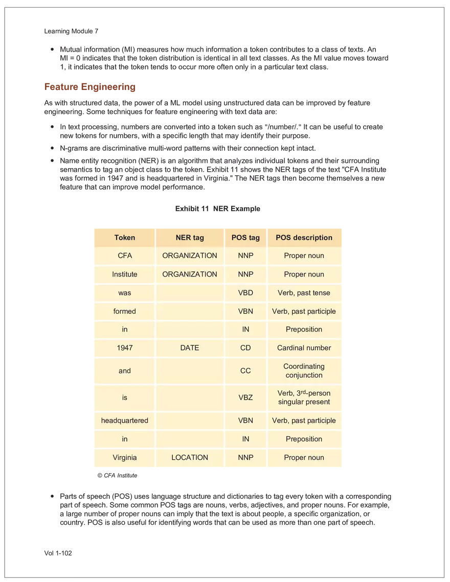
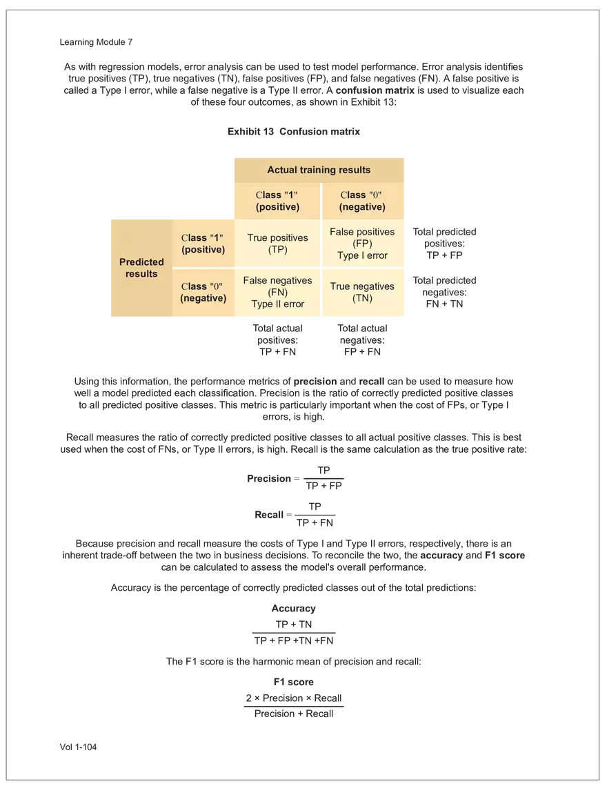
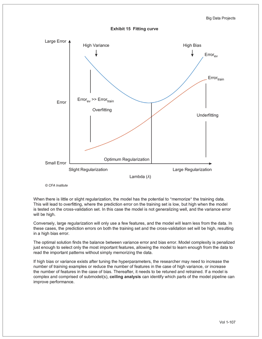
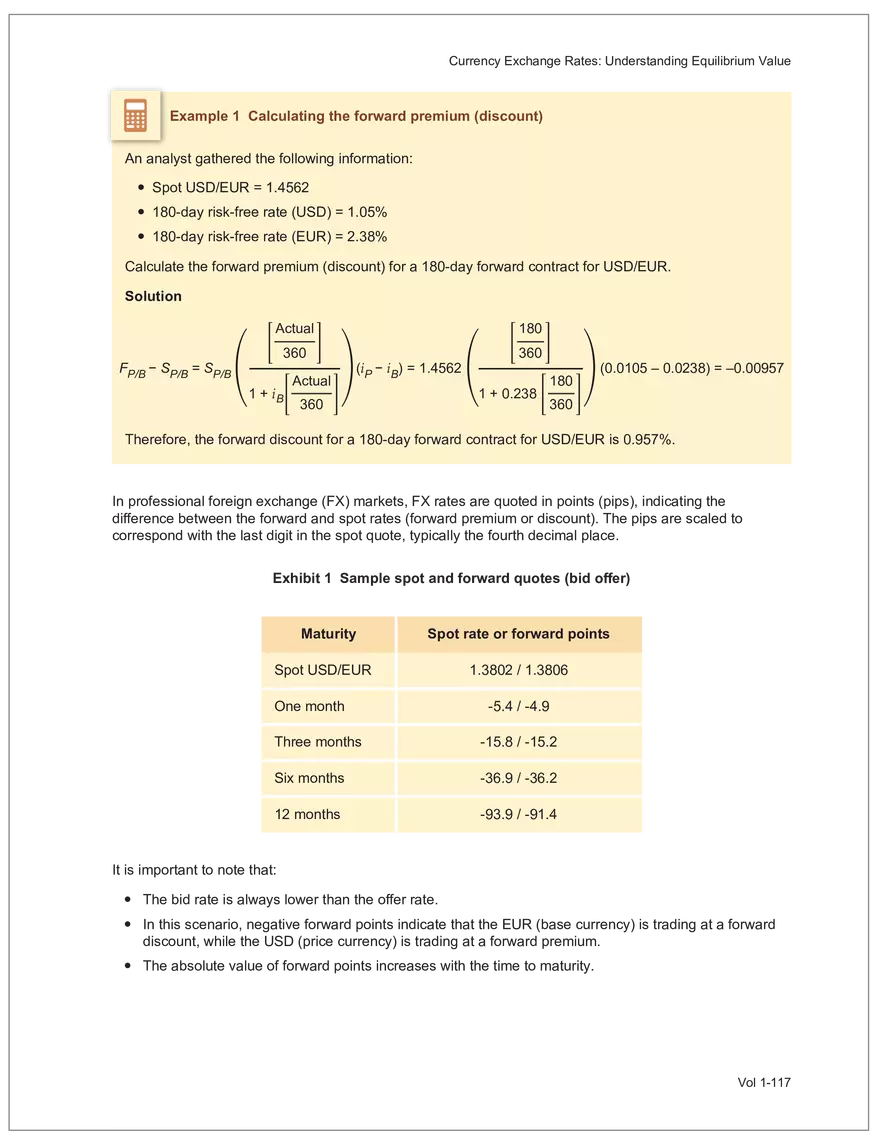
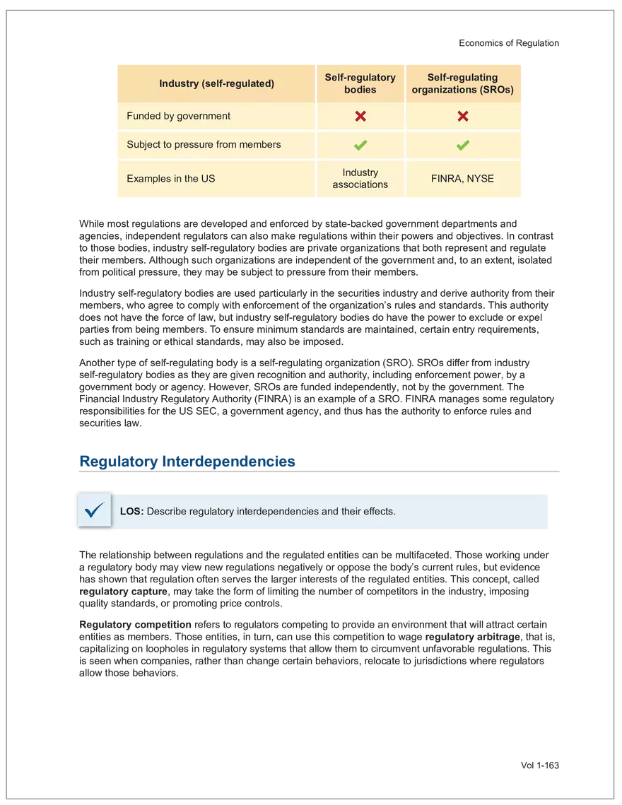
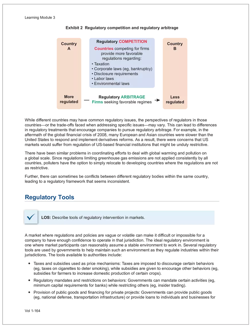
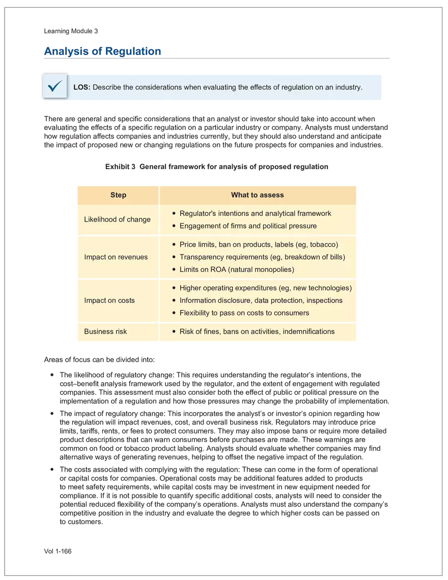
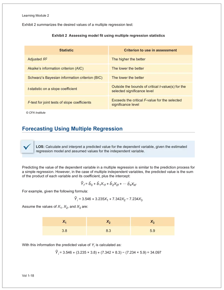
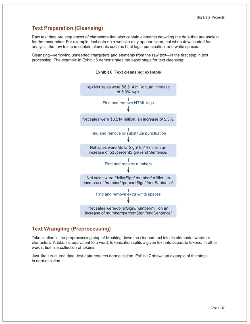
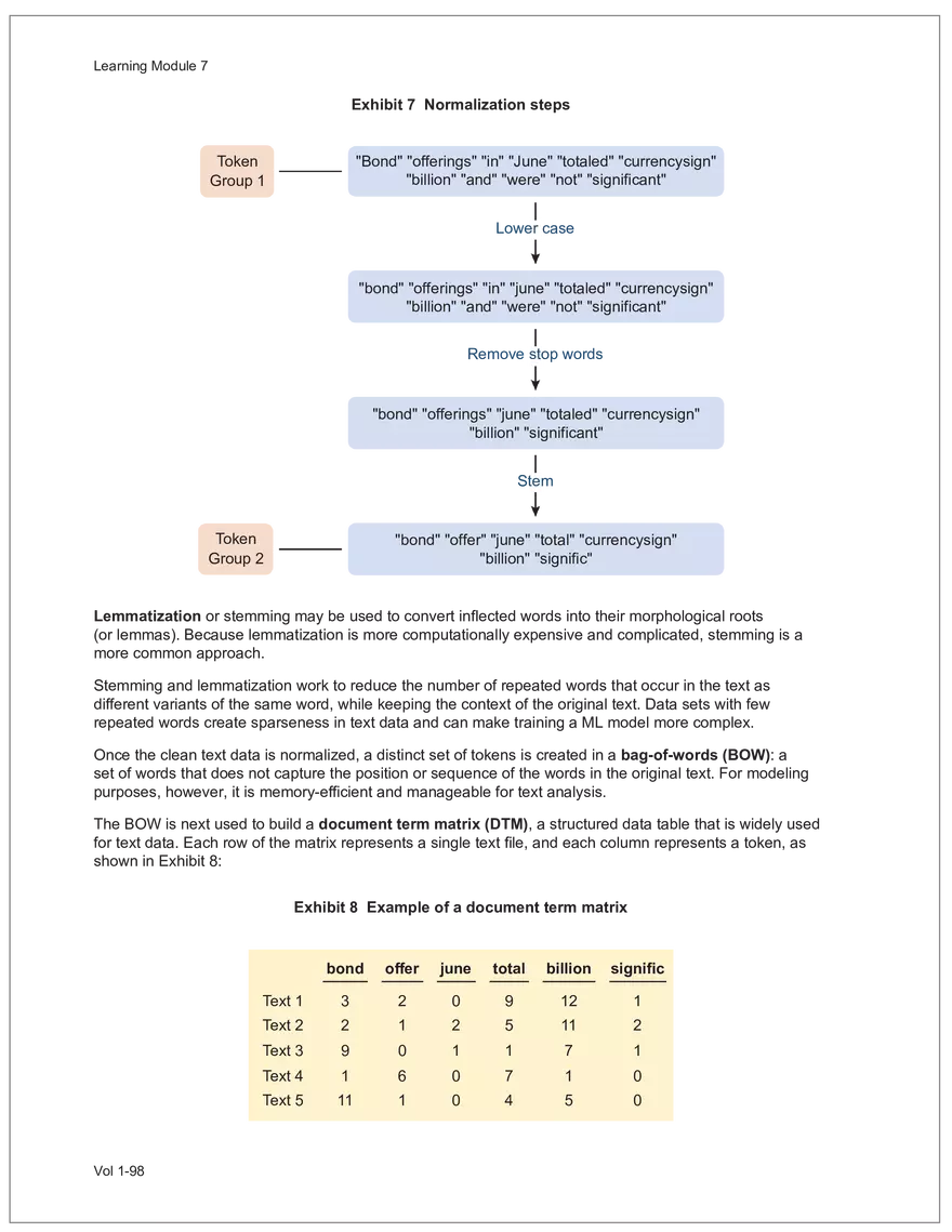
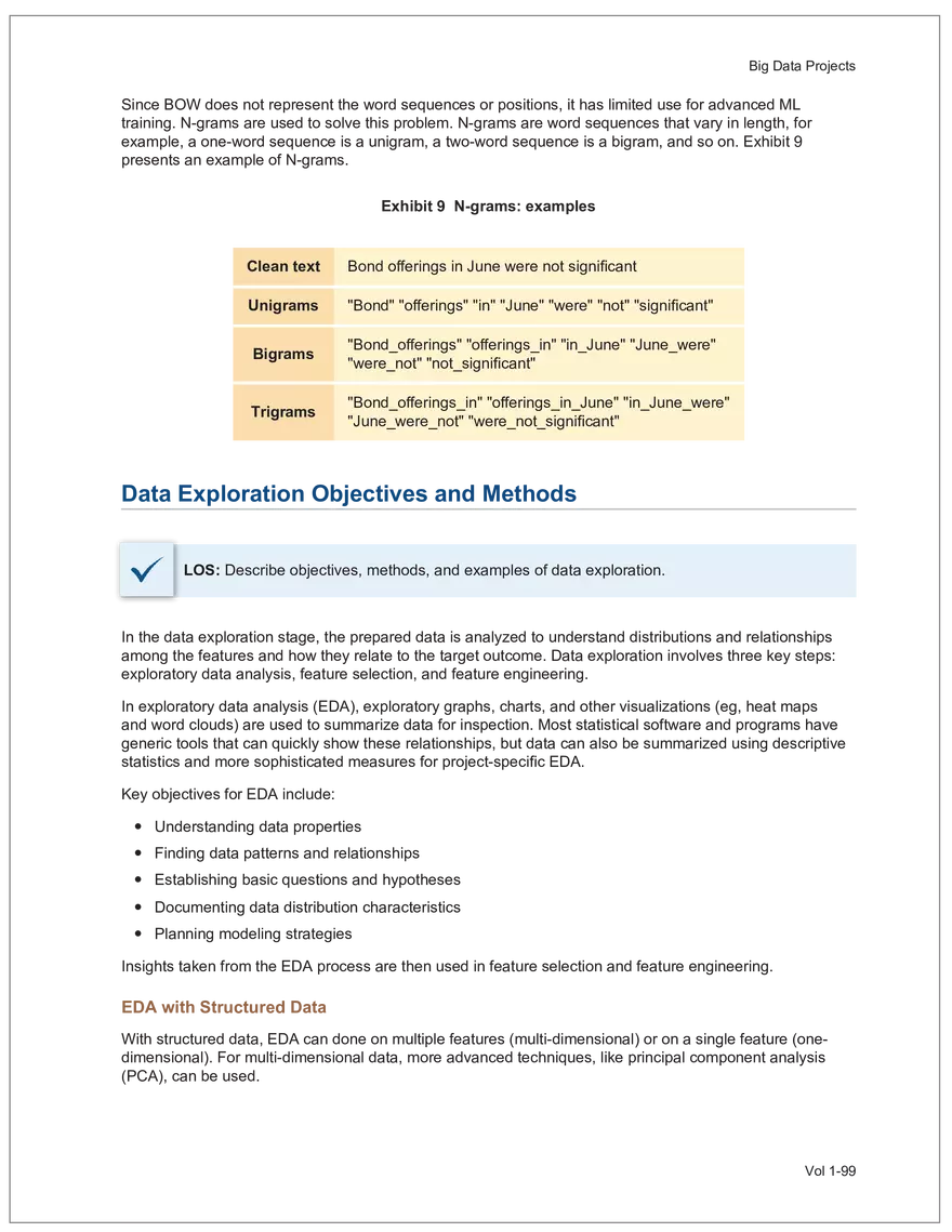
Find and remove HTML tags Net sales were $8,514 million, an increase of 5.3%. Find and remove or substitute punctuation Net sales were /dollarSign/ 8514 million an increase of 53 /percentSign/ /end Sentence/ Find and replace numbers Net sales were /dollarSign/ /number/ million an increase of /number/ /percentSign/ /endSentence/ Find and remove extra white spaces Net sales were/dollarSign//number/million an increase of /number//percentSign//endSentence/ Text Wrangling (Preprocessing) Tokenization is the preprocessing step of breaking down the cleaned text into its elemental words or characters. A token is equivalent to a word; tokenization splits a given text into separate tokens. In other words, text is a collection of tokens. Just like structured data, text data requires normalization. Exhibit 7 shows an example of the steps in normalization. Vol 1-97 Learning Module 7 Exhibit 7 Normalization steps Token Group 1 "Bond" "offerings" "in" "June" "totaled" "currencysign" "billion" "and" "were" "not" "significant" Lower case "bond" "offerings" "in" "june" "totaled" "currencysign" "billion" "and" "were" "not" "significant" Remove stop words "bond" "offerings" "june" "totaled" "currencysign" "billion" "significant" Stem Token Group 2 "bond" "offer" "june" "total" "currencysign" "billion" "signific" Lemmatization or stemming may be used to convert inflected words into their morphological roots (or lemmas). Because lemmatization is more computationally expensive and complicated, stemming is a more common approach. Stemming and lemmatization work to reduce the number of repeated words that occur in the text as different variants of the same word, while keeping the context of the original text. Data sets with few repeated words create sparseness in text data and can make training a ML model more complex. Once the clean text data is normalized, a distinct set of tokens is created in a bag-of-words (BOW): a set of words that does not capture the position or sequence of the words in the original text. For modeling purposes, however, it is memory-efficient and manageable for text analysis. The BOW is next used to build a document term matrix (DTM), a structured data table that is widely used for text data. Each row of the matrix represents a single text file, and each column represents a token, as shown in Exhibit 8: Exhibit 8 Example of a document term matrix bond offer june total billion signific Text 1 Text 2 Text 3 Text 4 Text 5 3 2 2 1 0 6 1 0 2 1 0 0 9 5 1 7 4 12 11 7 1 2 1 0 0 9 1 1 11 5 Vol 1-98 Big Data Projects Since BOW does not represent the word sequences or positions, it has limited use for advanced ML training. N-grams are used to solve this problem. N-grams are word sequences that vary in length, for example, a one-word sequence is a unigram, a two-word sequence is a bigram, and so on. Exhibit 9 presents an example of N-grams. Exhibit 9 N-grams: examples Clean text Unigrams Bond offerings in June were not significant "Bond" "offerings" "in" "June" "were" "not" "significant" "Bond_offerings" "offerings_in" "in_June" "June_were" "were_not" "not_significant" Bigrams Trigrams "Bond_offerings_in" "offerings_in_June" "in_June_were" "June_were_not" "were_not_significant" Data Exploration Objectives and Methods LOS: Describe objectives, methods, and examples of data exploration. In the data exploration stage, the prepared data is analyzed to understand distributions and relationships among the features and how they relate to the target outcome. Data exploration involves three key steps: exploratory data analysis, feature selection, and feature engineering. In exploratory data analysis (EDA), exploratory graphs, charts, and other visualizations (eg, heat maps and word clouds) are used to summarize data for inspection. Most statistical software and programs have generic tools that can quickly show these relationships, but data can also be summarized using descriptive statistics and more sophisticated measures for project-specific EDA. Key objectives for EDA include: y Understanding data properties y Finding data patterns and relationships y Establishing basic questions and hypotheses y Documenting data distribution characteristics y Planning modeling strategies Insights taken from the EDA process are then used in feature selection and feature engineering. EDA with Structured Data With structured data, EDA can done on multiple features (multi-dimensional) or on a single feature (onedimensional). For multi-dimensional data, more advanced techniques, like principal component analysis (PCA), can be used. Vol 1-99 Learning Module 7 For one-dimensional data, common summary statistics are used, such as mean, median, standard deviation, quartile ranges, skewness, and kurtosis. Data visualizations can also be created, such as histograms, density plots, bar charts, and box plots. Histograms use equal bins of values or value ranges to show the frequency of the data points in each bin, and thus show the distribution of the data. One-dimensional visualizations of multiple features are often stacked or overlaid on each other in a single plot for comparison. For example, density plots are smoothed histograms overlaid on standard histograms, used to understand the distribution of continuous data by normally distributing the mean, median, and standard deviation. To compare multiple features, multivariate data visualizations include stacked bar charts, multiple box plots, and scatterplots. Scatterplots are helpful to show the relationship between two variables. Feature Selection In the feature selection stage, the researcher selects the most pertinent variables for ML model training in order to simplify the model. Throughout the EDA stage, features that are both relevant and irrelevant are identified, but statistical diagnostics are used to remove redundancy, heteroskedasticity, and multicollinearity, with the goal of minimizing the number of features while also maximizing the predictive power of the model. Dimensionality reduction identifies features that account for the greatest variance between observations, reduces the volume of data, and creates new, uncorrelated combinations of features. But while both feature selection and dimensionality reduction reduce the number of features, neither involves altering the data. Feature Engineering Feature engineering produces new features derived from the given features to help better explain the data set. A ML model can only perform as well as the data used to train it, and feature engineering can improve the data by uncovering structures inherent, but not explicit, in the data. Techniques include altering, combining, or decomposing existing data. For example, for continuous data, a new feature may be just the logarithm of another, which is helpful if the data spans a large range or if the percentage differences are important. Other examples include bracketing by assigning a binary to a data point. converting categorical variables into a binary value; this is known as one hot encoding and is common in handling categorical data in ML. Unstructured Data: Text Exploration LOS: Describe objectives, methods, and examples of data exploration. LOS: Describe methods for extracting, selecting, and engineering features from textual data. Exploratory Data Analysis Text statistics vary by case and are used to analyze and reveal word patterns. Computing basic test statistics using tokens is known as term frequency (TF), which is the ratio of how often a particular token occurs to the total number of tokens in the data set. A collection of text data sets is called a corpus. Vol 1-100 For categorical data, new features can combine two features or decompose one feature into many, Big Data Projects Topic modeling is a text data application where the most informative words are identified by calculating methods such as a word cloud, which visualizes the most informative words and their TF values. Exhibit 10 is an example of a word cloud where the size of each word is decided by its TF value. Exhibit 10 Word cloud interpretation from Alphabet's 20XX 10-K filing Total revenue Result of operations Cost of revenue Google cloud Increase Fair value Effective tax rate Product mix Income tax Google search Marketable security Google service Foreign exchange effect Google playImpact of covid-19 Device mix Data center Paid click Data Currency exchange rate Distribution partner Net cash revenue US dollars Geographic mix Foreign currency Marketable equity security Financial result Content acquisition cost Marketing expenses Compensation expenses Purchase of property Feature Selection This stage removes a subset of tokens in the data with high TF values that are not material to the project. These stop words are taken out of the corpus to decrease vocabulary size, or the BOW, which makes the ML model simpler and thus more efficient, eliminating noisy features from the data set or tokens that detract from or fail to benefit ML model training. y Frequent tokens strain a ML model in deciding boundaries among texts, which causes model underfitting. y Rare tokens mislead a ML model into classifying texts that contain rare terms into a specific class, leading to model overfitting. To minimize the impacts of these data points, the researcher can use general feature selection methods for identifying and removing noisy features: y Frequency measures reduce vocabulary by filtering tokens with very high and low TF values. y Document frequency (DF) discards noisy features that carry no material information across all texts. The DF of a token is calculated as the number of documents that contain that token divided by the number of total documents in the data set. y Chi-square tests examine the independence of two events: occurrence of the token and occurrence of the class. The test ranks each token by its usefulness to each class in a text classification problem. Tokens with higher chi-square test statistics for a given class are more frequently associated and therefore have a higher discriminatory potential. Vol 1-101 TF. Using the TF, text statistics can be visually comprehended in the same way as structured data, using revenue percentage changes Information technology assets Advertising revenue Google network member Financial conditions revenue growth rate Cost Fair value Interest rate Learning Module 7 y Mutual information (MI) measures how much information a token contributes to a class of texts. An MI = 0 indicates that the token distribution is identical in all text classes. As the MI value moves toward 1, it indicates that the token tends to occur more often only in a particular text class. Feature Engineering As with structured data, the power of a ML model using unstructured data can be improved by feature engineering. Some techniques for feature engineering with text data are: y In text processing, numbers are converted into a token such as "/number/." It can be useful to create new tokens for numbers, with a specific length that may identify their purpose. y N-grams are discriminative multi-word patterns with their connection kept intact. y Name entity recognition (NER) is an algorithm that analyzes individual tokens and their surrounding semantics to tag an object class to the token. Exhibit 11 shows the NER tags of the text "CFA Institute was formed in 1947 and is headquartered in Virginia." The NER tags then become themselves a new feature that can improve model performance. Exhibit 11 NER Example Token CFA NER tag POS tag NNP NNP VBD VBN IN POS description ORGANIZATION Proper noun Institute ORGANIZATION was Proper noun Verb, past tense Verb, past participle Preposition formed in 1947 DATE CD Cardinal number Coordinating conjunction and is CC Ve rd rb, 3 -person VBZ singular present Verb, past participle Preposition headquartered in VBN IN Virginia LOCATION NNP Proper noun © CFA Institute y Parts of speech (POS) uses language structure and dictionaries to tag every token with a corresponding part of speech. Some common POS tags are nouns, verbs, adjectives, and proper nouns. For example, a large number of proper nouns can imply that the text is about people, a specific organization, or country. POS is also useful for identifying words that can be used as more than one part of speech. Vol 1-102 Big Data Projects Model Training, Structured versus Unstructured Data, and Method Selection LOS: Describe objectives, steps, and techniques in model training. Once the features are selected, the ML model can be trained. The training process is systematic, iterative, and recursive and can become fairly complex. The nature of the problem at hand, the input data available, and the level of performance needed to apply the model dictate that complexity. However, all ML model training involves three tasks: method selection, performance evaluation, and tuning. Method Selection There are no set guidelines on which method to fit a model with. However, there are a few factors that steer the researcher toward a broader process: y Supervised or unsupervised learning: Supervised models have a ground truth, or a target dependent variable that adds structure to the model. They can aim to predict a continuous value (regression) or a set classification of a dependent variable. Unsupervised learning aims to reduce the number of features that define the data set and group data points by similarities not immediately evident in the data. y Type of data, such as numerical, text, images, or speech y Size of data, including both the number of instances and features Further complicating the model selection process are data sets with mixed inputs (eg, both numerical and text data or both structured and unstructured data). In these cases, the results of one model can be used as an input for another model. Performance Evaluation Measuring a model's performance is a critical step in assessing its goodness of fit. For models that predict continuous variables, analysis of the error terms is used to measure fit. However, for binary classification models, there are several techniques available to assess performance. Exhibit 12 shows three of these techniques. Exhibit 12 Techniques of ML performance evaluation y Actual vs. predicted results (confusion matrix) Error analysis y Metrics: precision, recall, accuracy, and F1 score y Trade-off between false and true positive rates y Distinct cutoff points and areas under the curve (AUC) y Greater AUC (closer to 1) means better performance Receiver operating characteristic (ROC) y Appropriate for continuous data and regressions y Measures all prediction errors Root mean square error (RMSE) y Smaller RMSE means better performance Vol 1-103 y True/false positives/negatives: TP, FP, FN, TN Learning Module 7 As with regression models, error analysis can be used to test model performance. Error analysis identifies true positives (TP), true negatives (TN), false positives (FP), and false negatives (FN). A false positive is called a Type I error, while a false negative is a Type II error. A confusion matrix is used to visualize each of these four outcomes, as shown in Exhibit 13: Exhibit 13 Confusion matrix Actual training results Class "1" Class "0" (positive) (negative) False positives (FP) Type I error Total predicted positives: Class "1" (positive) True positives (TP) TP + FP Predicted results False negatives (FN) Type II error Total predicted negatives: FN + TN Class "0" (negative) True negatives (TN) Total actual positives: TP + FN Total actual negatives: FP + FN Using this information, the performance metrics of precision and recall can be used to measure how well a model predicted each classification. Precision is the ratio of correctly predicted positive classes to all predicted positive classes. This metric is particularly important when the cost of FPs, or Type I errors, is high. Recall measures the ratio of correctly predicted positive classes to all actual positive classes. This is best used when the cost of FNs, or Type II errors, is high. Recall is the same calculation as the true positive rate: TP Precision = TP + FP TP Recall = TP + FN Because precision and recall measure the costs of Type I and Type II errors, respectively, there is an inherent trade-off between the two in business decisions. To reconcile the two, the accuracy and F1 score can be calculated to assess the model's overall performance. Accuracy is the percentage of correctly predicted classes out of the total predictions: Accuracy TP + TN TP + FP +TN +FN The F1 score is the harmonic mean of precision and recall: F1 score 2 × Precision × Recall Precision + Recall Vol 1-104 Big Data Projects The F1 score is the more appropriate of the two when there is an unequal distribution across the classes and finding the equilibrium between the two is needed. Receiver operating characteristic (ROC) involves plotting a curve showing the trade-off between the false positive rate (x-axis) and true positive rate (y-axis). Area under the curve (AUC) measures the area under the ROC curve. An AUC of 1.0 indicates perfection, while an AUC below 0.5 indicates random guessing. The ROC curve becomes more convex with respect to the true positive rate as AUC increases, as shown in Exhibit 14. Exhibit 14 Area under the curve (AUC) for different receiver operating characteristic (ROC) curves True positive 1.0 rate (TPR) Model Y AUC = 80% 0.8 0.6 0.4 0.2 0.0 Model X AUC = 95% Model Z AUC = 70% Random guess AUC = 50% 0.0 0.2 0.4 0.6 0.8 1.0 False positive rate (FPR) For a continuous data set, the root mean squared error (RMSE) metric can be used to assess a model's performance. The RMSE captures all the prediction errors in the data (n) and is mostly used for regression methods. The formula for RMSE is: RMSE (Predicted − Actual ) i i �� n Vol 1-105 Learning Module 7 Tuning LOS: Describe objectives, steps, and techniques in model training. Once a model's performance has been evaluated, steps can be taken to improve its performance. A high prediction error on the training set indicates that the model is underfitting, while higher prediction errors on the cross-validation set compared with the training set tell the researcher that the model is overfitting. There are two types of errors when model fitting: y Bias error is high when the model underfits the training data. This generally occurs when the model is underspecified and the model is not adequately learning from the patterns in the training data. In these cases, both the training set prediction errors and cross-validation errors will be large. y Variance error is high when the model overfits to the training data, or the model is overly complicated. The training set prediction error will be much lower than on the cross-validation set. Neither of these errors can be completely eliminated, but the trade-off between the two errors should minimize the aggregate error over the data series. Balance is necessary to finding the optimal model that neither underfits nor overfits. Finding the correct model parameters, such as regression coefficients, weights in neural networks (NNs), and support vectors in support vector machines, is critical to properly fitting a model. The model parameters are dependent on the training data and are learned during the training process through optimization techniques. Hyperparameters are not dependent on training data and are used for estimating model parameters. Examples of these include the regularization term (λ) in supervised models, activation function and number of hidden layers in NNs, number of trees and tree depth in ensemble methods, k in k-nearest neighbor classification and k-means clustering, and p-threshold in logistic regression. Researchers optimize hyperparameters based on tuning heuristics and grid searches rather than using an estimation formula. A grid search is a method for training ML models through combinations of hyperparameter values and cross-validation to produce optimal model performance (training error and cross-validation error are close), which leads to a lower probability of overfitting. The plot of training errors for each hyperparameter is called a fitting curve, shown in Exhibit 15: Vol 1-106 Big Data Projects Exhibit 15 Fitting curve Large Error High Variance High Bias Errorev Error train Error >> Error E ev train rror Overfitting Underfitting Optimum Regularization Slight Regularization Small Error Large Regularization Lambda (λ) © CFA Institute When there is little or slight regularization, the model has the potential to "memorize" the training data. This will lead to overfitting, where the prediction error on the training set is low, but high when the model is tested on the cross-validation set. In this case the model is not generalizing well, and the variance error will be high. Conversely, large regularization will only use a few features, and the model will learn less from the data. In these cases, the prediction errors on both the training set and the cross-validation set will be high, resulting in a high bias error. The optimal solution finds the balance between variance error and bias error. Model complexity is penalized just enough to select only the most important features, allowing the model to learn enough from the data to read the important patterns without simply memorizing the data. If high bias or variance exists after tuning the hyperparameters, the researcher may need to increase the number of training examples or reduce the number of features in the case of high variance, or increase the number of features in the case of bias. Thereafter, it needs to be retuned and retrained. If a model is complex and comprised of submodel(s), ceiling analysis can identify which parts of the model pipeline can improve performance. Vol 1-107 Learning Module 7 Vol 1-108 Economics Learning Module 1 Currency Exchange Rates: Understanding Equilibrium Value LOS: Calculate and interpret the bid-offer spread on a spot or forward currency quotation and describe the factors that affect the bid-offer spread. LOS: Identify a triangular arbitrage opportunity and calculate its profit, given the bid-offer quotations for three currencies. LOS: Explain spot and forward rates and calculate the forward premium/discount for a LOS: Calculate the mark-to-market value of a forward contract. LOS: Explain international parity conditions (covered and uncovered interest rate parity, forward rate parity, purchasing power parity, and the international Fisher effect). LOS: Describe relations among the international parity conditions. LOS: Evaluate the use of the current spot rate, the forward rate, purchasing power parity, and uncovered interest parity to forecast future spot exchange rates. LOS: Explain approaches to assessing the long-run fair value of an exchange rate. LOS: Describe the carry trade and its relation to uncovered interest rate parity and calculate the profit from a carry trade. LOS: Explain how flows in the balance of payment accounts affect currency exchange rates. LOS: Explain the potential effects of monetary and fiscal policy on exchange rates. LOS: Describe objectives of central bank or government intervention and capital controls and describe the effectiveness of intervention and capital controls. LOS: Describe warning signs of a currency crisis. Foreign Exchange Market Concepts LOS: Calculate and interpret the bid-offer spread on a spot or forward currency quotation and describe the factors that affect the bid-offer spread. An exchange rate represents the price of one currency in terms of another currency. It is stated as the number of units of a particular currency (the price currency) required to purchase one unit of another currency (the base currency). Vol 1-111 given currency. Learning Module 1 CFA curriculum uses the convention P/B: the number of units of the price (P) currency needed to purchase one unit of the base (B) currency. For example, suppose the USD/GBP exchange rate is currently 1.5125. From this exchange rate quote, we can infer the following: y 1 GBP will buy 1.5125 USD. y A decrease in the exchange rate (eg, from 1.5125 to 1.5120) means that 1 GBP will be able to purchase fewer USD. ○ Fewer USD will now be required to purchase 1 GBP (ie, the cost of 1 GBP has fallen). ○ This decrease in the exchange rate means that the GBP has depreciated (ie, lost value) against the Just like the price of any product, the price reflected in an exchange rate is the amount of the numerator Spot exchange rates (S) are quotes for transactions that call for immediate delivery. For most currencies, immediate delivery means “T + 2” (ie, the transaction is settled 2 days after the trade is agreed upon by the parties). In professional FX markets, an exchange rate is usually quoted as a two-sided price. Dealers typically quote both a bid price (ie, the price at which they are willing to buy) and an offer price (ie, the price at which they Bid-offer quotes in foreign exchange have two main points: y The offer price is higher than the bid price, which creates the bid-offer spread, a compensation for providing foreign exchange. y Requesting a two-sided quote from the dealer allows a choice between whether the base currency will be bought (ie, paying the offer) or sold (ie, hitting the bid). This choice provides flexibility in transactions. In FX, dealers have two pricing levels: one level for clients and another for the interbank market. Dealers engage in currency transactions among themselves in the interbank market in order to adjust their inventories and risk positions, distribute foreign currencies to clients, and transfer FX rate risk to willing market participants. This global network handles large transactions, typically over 1 million units of the base currency; nonbank entities like institutional asset managers and hedge funds can also access the network. The bid-offer spread that dealers provide to clients is typically wider than what is observed in the interbank market. The bid-offer spread is sometimes measured in points, or pips, which are scaled to the last digit in the spot exchange rate quote. Exchange rates for most currency pairs (except those involving the Japanese yen) are quoted to four decimal places. For example, the bid-offer spread in the interbank market for USD/EUR might be 1.2500–1.2504. This is a difference of 0.0004, or 4 pips, while a dealer’s spread for the same currency pair may be 0.0006, or 6 pips. The bid-offer spread in the FX market, as quoted to dealers’ clients, can vary widely among different exchange rates and can change over time, even for a single exchange rate. The spread size is primarily influenced by the bid-offer spread in the interbank market, transaction size, and the relationship between the dealer and the client. A client’s creditworthiness can also be a factor, although, given the short settlement cycle in the spot FX market, credit risk is not the primary determinant of bid-offer spreads.